Download
1 / 6
60 likes | 189 Views
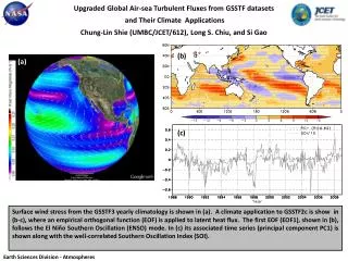
This study investigates the impact of subtle alterations in land surface models (LSMs) on atmospheric conditions, utilizing NASA's Goddard Multi-Scale Modeling Framework (MMF) coupled with the multi-model Land Information System (LIS). By comparing two versions of the NCAR Common Land Model (CLM), we demonstrate how changes in land-atmosphere interactions influence regional pressure patterns and circulation. The models reveal significant divergence in temperature and radiation patterns within just a few days, highlighting the importance of accurately simulating local processes for global climate predictions.

E N D
Exploring Local Land Surface Feedbacks to Regional CirculationKaren Mohr1, Jiun-Dar Chern1,2, Wei-Kuo Tao1, Code 612, 1NASA GSFC and 2Morgan State • General circulation models are typically coupled to a single land surface model (LSM). New versions of coupled modeling systems that incorporate new physics in both models make it difficult to isolate signals from the new LSM physics. We used the free-running Goddard Multi-Scale Modeling Framework (MMF) coupled to the multi-model Land Information System (LIS) to see if subtle changes to an LSM would feedback to the atmosphere at regional scales and how quickly that would happen. • The Goddard MMF-LIS is a GCM with arrays of 2-D cloud-resolving models replacing the moist physics parameterization, allowing true, global cloud-resolving capability. • The tested LSM is the NCAR Common Land Model (CLM) 2.0 and its update, CLM 2.1, that incorporates improvements in the soil-to-atmosphere heat transfer, but not in other areas. • By incorporating both models in LIS, it is possible to have identical initial atmospheric conditions. • Differences in regional pressure patterns due to local feedbacks among the shortwave radiation fluxes, land surface heat fluxes, and cloud amounts emerged after 10-14 days. a) d) e) b) f) c) CLM 2.0 (Original) CLM 2.1 (Modified) g) Figure 1:North American regional maps of 200 mb temperatures (a-c) and sea level pressures (d-f) for the CLM 2.0 (black line) and CLM 2.1 (red line) simulations after 5 days (a, d), 10 days (b, e), and 15 days (c, f). Panel g) is the time series of SW downward radiation for a gridcell centered at 26°N 102.5°W (Central Mexico), illustrating that differences at the local scale emerge very quickly in the simulation (< 2 days). Earth Sciences Division - Atmospheres
Name: Karen Mohr, NASA/GSFC, Code 612 E-mail: karen.mohr-1@nasa.gov Phone: 301-614-6360 References: Mohr, K.I., W.-K. Tao, J.-D. Chern, S.V. Kumar, and C. Peters-Lidard, 2012: The NASA-Goddard Multi-scale Modeling Framework-Land Information System: Global land/atmosphere interaction with resolved convection. Environmental Modeling and Software, 39, 103115. Tao, W.-K., J.-D. Chern, R. Atlas, D. Randall, M. Khairoutdinov, J.-L. Li, D.E. Waliser, A. Hou, X. Lin, C. Peters-Lidard, W. Lau, J. Jiang, and J. Simpson, 2009. A multiscale modeling system: Developments, applications, and critical issues. Bulletin of the American Meteorological Society, 90, 515-534. Data Sources: Parameter datasets for LIS include MODIS land cover classes, GTOPO30 elevations, FAO soil fractions maps. Forcing datasets on the GCM include NOAA weekly Reynolds Optimum Interpolation SST Analysis Ver. 2, and ozone product merging the NASA UARS measurements with the Atmospheric Model Intercomparison Project 2 ozone dataset. Validation and comparison datasets include MERRA, NCEP reanalysis, CMORPH rainfall, TRMM rainfall, FLUXNET surface fluxes. Technical Description of Figures: Figure 1: We conducted a free-running (no data assimilation) global simulation of 2007-2008 of MMF-LIS using two different versions of the Common Land Model (CLM 2.0 and 2.1) in LIS. Resolution of the GCM was 2.5°×2°, 4-km for the cloud resolving Goddard Cumulus Ensemble arrays. In CLM 2.1, the changes to the model physics are the computation of atmospheric forcing height, vegetation temperature, canopy interception of precipitation, and the drag coefficient between the underlying soil (or canopy surface) and the canopy air. All four of these state variables are used in determining the soil heat transfer to the atmosphere. Both simulations, CLM 2.0 and CLM 2.1, start with identical initial conditions and identical atmospheric model physics. The regional maps show how quickly the simulated North American regional circulations diverge after initialization. Subtle differences between the two simulations appear by Day 5 at 200 mb and Day 10 for the sea level pressures. By Day 15, there are substantial differences in the locations, orientations, and magnitudes of all cyclones/troughs and anticyclones/ridges in the region. At the local scale for a region in Central Mexico, differences between the two versions begin to emerge on 2 Jan. By 3 Jan, the difference in the daily maximum shortwave downward radiation is more than 300 W m-2 because there is significantly more total cloud cover (not shown) and daily maximum surface temperatures 5K-10K lower (not shown) in the CLM 2.1 simulation due to a slower soil-to-atmosphere heat transfer. As most GCMs are coupled to a single land surface model, a singular advantage provided by LIS is the ability to run multiple land surface models, i.e., ensemble land surface modeling within the same global model framework. The differences between the MMF-LIS panels demonstrate global sensitivity to integrated local-scale land surface processes. Scientific significance: Improved representation of the water and energy cycles is critical to global weather and climate simulation. The MMF-LIS explicitly accounts for km-scale cloud and land surface processes. This model framework concept shows promise in improving the simulation of global precipitation and thus atmospheric circulations at multiple scales without significant increases in computational overhead. Relevance for future science and relationship to Decadal Survey: The Goddard MMF and its constituent models have given us new insight into multi-scale land-atmosphere interactions and precipitation processes in support of the basic science goals of the NASA Energy and Water Cycle Study (NEWS), Modeling Analysis, and Prediction (MAP) program, and the Precipitation Measuring Mission. In addition to process studies in water and energy cycles, the MMF is used for GPM algorithm support in areas where the satellite data record is thin (e.g., high latitudes). Earth Sciences Division - Atmospheres
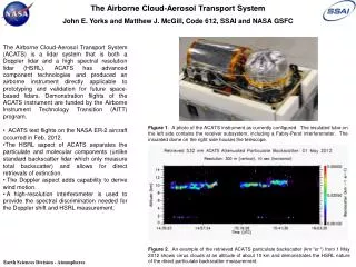
A Novel Technique to Retrieve Cloud Ice Water from Microwave Humidity Sounder Jie Gong (USRA), Dong L. Wu, Code 613, NASA GSFC Ice water path (IWP) is a key variable to determine cloud radiative and thermodynamical properties in Earth climate systems. Substantial uncertainties remain among IWP measurements from satellite sensors, largely due to the different assumptions made about cloud microphysics in the retrievals. In this study, we develop an IWP retrieval algorithm from the Microwave Humidity Sounder (MHS) high-frequency channel radiances constrained by CloudSat Cloud Profiling Radar cloud ice measurements. The retrieved IWP provides CloudSat-consistent measurements of ice water amount in thick/dense ice clouds and floating snows. Cloud-induced radiance depression (Tcir) is the radiance difference between the measured and expected clear-sky background. We compiled 5-yr of collocated and coincident NOAA-18 MHS and CloudSat scenes to build the empirical Tcir-IWP model for 157 and 183 GHz channels (Fig. 1a), which is also dependent on cloud top height. The IWP retrieval from this empirical algorithm is consistent with CloudSat in terms of cloud ice map and normalized probability density distribution (PDF) (Fig. 1b and Fig. 2a,c). Mesoscale model simulations suggest that MHS-observed IWP in the tropics is mostly precipitating ice, which can be used to infer floating snow precipitation in the future (Fig. 1b). (b) (a) CloudSat WRF, ice cloud + floating snow NOAA operational product WRF, ice cloud only MHS retrieval Fig. 1: (a) 2D probability density functions (PDFs) of collocated and coincident CloudSat IWP and MHS 190 GHz Tcir measurements from near-nadir views (color shades) with peaks marked by black dots and the retrieval curve in red. (b) PDF of a month of retrieved MHS IWP (red) compared with CloudSat (black), operational product (cyan) and model simulation (green). (c) (b) (a) Fig. 2: IWP (a) and cloud top height (c) retrievals for Hurricane Earl on Aug. 31, 2010 from NOAA-18 MHS with simultaneous CloudSat overpasses. (b) is from NOAA operational IWP product. The CloudSat overpass is plotted in crosses. Earth Sciences Division - Atmospheres
Name: Jie Gong, NASA/GSFC Code 613 E-mail:Jie.Gong@nasa.gov Phone: 301-614-6154 References: Gong, J. and D. L. Wu: CloudSat-constrained cloud ice water path and cloud top height retrievals from MHS 157 and 183 GHz radiances, in submission to Atmos. Meas. Tech. Wu, D. L., R. T. Austin, M. Deng, S. L. Durden, A. J. Heymsfield, J. H. Jiang, A. Lambert, J.-L. Li, N. J. Livesey, G. M. McFarquhar, J. V. Pittman, G. L. Stephens, S. Tanelli, D. G. Vane, and D. E. Waliser: Comparisons of global cloud ice from MLS, Cloud- Sat, and correlative data sets, J. Geophys. Res., 114(D00A24), doi:10.1029/2008JD009946, 2009. Acknowledgement: This work is supported by NASA NNH10ZDA001N-ESDRERR project. Mesoscale model (WRF) simulations are provided by Prof. Varavut Limpasuvan from Coastal Carolina University, SC. Free online resources of CRTM and AAPP software and MERRA analysis products are highly appreciated. Data Sources: CloudSat 2B-CWC-RO IWC product (R04) and NOAA-18 MHS L1B radiance data between June, 2006 and March, 2011. MERRA 1.25° X 1.25° 3-hourly assimilation products for the same period of time. Technical Description of Figures: Figure 1: (a) MHS Tcir is calculated by subtracting corresponding clear-sky radiance (Tccr) from the observed radiance (Tb). Tccr is computed using Community Radiative Transfer Model (CRTM) and MERRA analysis products. Collocation (coincident) is defined such that CloudSat and MHS footprints are separated by no more than 10 km in space (15 mins in time). The saturation Tcir is estimated from the lowest value that has been observed during the entire period. The retrieval line is regressed over the peak of 2D PDF use the form Tcir = Tcir0{1-exp[-IWP/(c0+c1ht+c2ht2)]}, where ht is cloud top height, and Tcir0, c0, c1 and c2 are evaluated from three groups of CloudSat IWP with separating ht into 10, 12 and 14 km bins. Sequential approach is applied for the joint retrieval afterwards to retrieve IWP and ht simultaneously. (b) August, 2010 is selected to compute the monthly PDFs from CloudSat and NOAA-18 MHS. Red dots are from raw retrievals and red solid line is quality-controlled. WRF simulations are only carried out on Aug.1-2, 15-16, and 30-31, 2010. The horizontal resolution is 3 km with cumulus parameterization being turned-off. Results from a relative coarse resolution (10 km, not shown) are very similar. Green dashed line is from WRF ice clouds only, which diminish at larger IWP values, while PDF computed from WRF floating snow (green dash-dot line) agrees with CloudSat and MHS retrievals the most. Figure 2: The current retrieval algorithm is valid for clouds with ht < 18 km that locate in the tropics [30°S, 30°N]. This algorithm can be extended to higher latitudes by allowing the Tcir-IWP relationship to vary with temperature lapse rate, which we are currently working on. Scientific Significance: This novel algorithm substitutes traditional 89 GHz channel with 183.3 GHz channels, the latter of which is not sensitive to water clouds and less sensitive to surface signals. Therefore, this algorithm is fast, reliable, and highly consistent with CloudSat measurements, yet outperforms CloudSat because of its wide swath width, long-time duration and frequent daily sample rate. Relevance for Future Science and NASA missions: As MHS and its former version (AMSU-B) have been aboard on a series of satellites, they provide us unprecedented opportunities to carry out research on weather (e.g., hurricane, cloud diurnal cycle) and climate (e.g., IWP long-term trend). Cross-instrument consistent IWP observations will greatly help to constrain and improve model ice clouds. Our empirical cloud ice scattering model can be easily applied to other instruments with high-frequency microwave channels, such as NPP ATMS and GPM GMI. The combination of all sensors will provide real-time IWP monitoring at almost every corner of the globe. Earth Sciences Division - Atmospheres
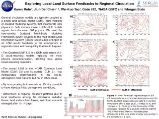
DISCOVER-AQ San Joaquin Valley California Winter 2013 CampaignKen Pickering, Code 614, Brent Holben, Code 618, NASA GSFC; Jim Crawford, NASA LaRC DISCOVER-AQ completed its second deployment in a series of four airborne campaigns aimed at improving the use of satellite observations to diagnose near-surface air quality. The target was California’s central valley during winter where cold, stagnant conditions encourage the accumulation of fine particles to reach unhealthy levels. Airborne sampling was conducted in coordination with ground monitoring sites operated by the state and local air pollution agencies. The NASA P-3B conducted spiral profiles for in-situ aerosol and trace gas data collection over six of these sites and two additional missed-approach airport sites (Figure 1), each of which was outfitted with AERONET sun photometers for aerosol optical depth (AOD) measurements. The NASA King Air carried a High Spectral Resolution Lidar (HSRL) for observations of aerosol optical properties and their vertical distribution. The first five flights documented a period of pollution build-up as particulate levels in the southern end of the valley tripled. A second period of build-up was observed with the remaining flights. Figure 3 shows similarity in the trends of the two measurements, which is encouraging for applicability of observations of AOD from satellite for surface air quality. An important factor in these intense pollution episodes was the shallowness of the polluted layer which was almost always limited to the lowest 2000 feet above the surface. Earth Sciences Division - Atmospheres Tranquility Fresno Hanford Huron Visalia Corcoran Porterville Bakersfield Palmdale Figure 2: NASA P-3B aircraft at low altitude during a missed approach at the Visalia Airport in the California campaign. Figure 1: Flight tracks for the NASA P-3B aircraft over the San Joaquin Valley of California. Spiral profile and missed approach locations labelled in red. Figure 3: Time series of the trend in surface PM2.5 (partic- ulate matter with diameter < 2.5 micrometers) and aerosol optical depth (AOD) from the sun photometer at Bakers- field during the first aerosol pollution episode documented during the San Joaquin Valley campaign. Note that the AOD generally follows the trend of surface PM2.5 during the development of the pollution episode. White bars indicate time periods of research flights. Colored lines indicate various pollution threat levels, with orange indicating the 24-hr average air quality standard.
Name: Dr. Kenneth E. Pickering, Code 614 E-mail: Kenneth.E.Pickering@nasa.gov Phone: 301-614-5986 References: No papers resulting from the DISCOVER-AQ (Deriving Information on Surface Conditions from Column and Vertically-Resolved Observations Relevant to Air Quality) California campaign as yet. Other scientists conducting DISCOVER-AQ measurements (not a complete listing) include: Scott Janz (Code 614), Jay Herman (UMBC, Code 614); Chris Hostetler, Rich Ferrare, Bruce Anderson (NASA LaRC) Data Sources: MODIS AOD, OMI NO2 and O3, AERONET AOD, Pandora NO2 and O3 columns Technical Description of Figures: Figure 1: Map showing P-3B flight tracks from Palmdale, CA base into the San Joaquin Valley, as well as to more distant locations in the San Francisco Bay area and offshore of Los Angeles. The northern track was designed to investigate transport into the San Joaquin Valley from the Bay Area. The flights off the coast were in support of the ER-2-based PODEX mission. Spiral profiles were conducted at Bakersfield, Porterville, Hanford, Huron, Tranquility, and Fresno. Missed approaches were conducted at Bakersfield, Porterville, Corcoran, Hanford, Fresno, and Visalia. Figure 2: The NASA P-3B performing a missed approach at the Visalia Airport. The missed approaches enabled profiling down to approximately 100 feet above the ground, which was critical for characterizing the composition of the rather shallow boundary layer (seldom deeper than 2000 ft.), as the spirals were limited to a base altitude of 1000 ft. over populated areas and 500 ft. over rural regions. Figure 3: Time series of PM2.5 from surface monitor operated by the local air pollution agency and aerosol optical depth (AOD) from a co-located AERONET sun photometer at Bakersfield. Time series extends from January 16 to 24, 2013. While the trend over this entire time period is similar from the two instruments, trends from the two instruments within particular days show differences largely due to evolution of boundary layer depth. Due to the shallowness of the mixed layer, the AOD values in this campaign were relatively modest. The values found here are often exceeded in areas that are not experiencing as high loading of fine particles at the surface, but have deeper mixing. Scientific significance: Statistical analyses of the data from the California campaign will more formally examine the linkage between surface and column observations, not only for aerosols, but also for the trace gases O3, NO2, and HCHO. These analyses will yield information on how well the column measurements from satellite represent surface air quality. The measurements also allow assessment of the magnitude of horizontal and vertical variability of aerosols and trace gases. The data are extremely useful for evaluating regional air quality models. Relevance for future science and relationship to Decadal Survey: DISCOVER-AQ data are extremely useful in planning future geostationary satellites. A key advantage of geostationary platforms is the ability to obtain many observations of gases and aerosols throughout the day. The DISCOVER-AQ data are collected throughout the daytime hours to allow determination of the temporal changes occurring in the study regions that a future satellite must be able to detect. Assessment of the horizontal and vertical variability of gases and aerosols has a direct bearing on determining the resolution needed for both satellite instruments and air quality models. The DISCOVER-AQ data and subsequent analyses support the planning for the Geostationary Coastal and Air Pollution Events (GEO-CAPE) satellite, which was proposed as a Tier II mission by the National Research Council’s Earth Science Decadal Survey. Earth Sciences Division - Atmospheres