Risk Modeling
360 likes | 385 Views
Understand risk modeling techniques and decision-making strategies for parameters with probability distributions. Explore ways to deal with risk and optimize expected returns. Learn about different model types and methods to incorporate risk in objective functions.

Risk Modeling
E N D
Presentation Transcript
Risk Modeling Chapter 20
What is "risk"? Some outcomes, such as yields or prices, are not known with certainty. In risk modeling, we often assume that the distribution of a parameter is known with certainty, even if a particular observation's value is not known with certainty. Risk modeling techniques are designed to give a robust solution to a problem involving parameters with probability distributions.
Ways to deal with risk • Ignore it. Not always a good option! • Assume producers are risk neutral and maximize expected returns, deal with risk only as it affects transitions from a one state of nature to the next over time. (A complicated topic.). • Assume producers respond to risk as well as expected returns.
Risk, Decision Making, and Recourse • Fundamental distinction between cases: • All decisions must be made now with • uncertain outcomes resolved later, after • all random draws from the distribution have • been taken. • Some decisions are made now, then after • some uncertainties are resolved, other • decisions are made later.
Examples 1) Invest at the beginning of the year, discover returns at end of year with no intermediate buying or selling decisions. 2)Invest at the beginning of the year, buy or sell during the year depending on stock prices.
Model Types The first type of model is very common and is generally called a stochastic programming model. The second type is called stochastic programming with recourse.
Aside: "Discounting" Coefficients Data for LP models are almost never certain. Rather than use the expected mean of a stochastic coefficient, a conservative approach is taken in a "deterministic model." Objective function revenue coefficients may be deflated while cost coefficients are inflated. The difficulty with this approach is the resulting probability of the solution. Conservative estimates on all parameters can imply a highly unlikely outcome and yield overly conservative decisions.
Modeling Risk in the Decision Process • Put both the expected returns and some representation of risk in the objective function, with weights. • Maximize expected returns subject to a limit on variability. • Minimize variability subject to an income target. • Hybrids.
Quadratic Programming and Risk Modeling • Quadratic programming can be used • for mean-variance analysis (Freund). • Max jcjXj - jkSjkXjXk • s.t. jaijXj bj for all j constraints • is a parameter representing degree of risk aversion. cj is expected return. The Sjk are elements of the variance-covariance matrix for the income of the alternatives.
Matrix Notation Max C X - X'SX s.t AX b (X non-negative)
Portfolio Analysis The model becomes: Max jcjXj - jkSjkXjXk s.t. jXj = 1 The Xj represent the way the total portfolio dollars should be divided among alternative investments.
Markowitz's E-V Formulation Min X'SX s.t. CX = AX b is the income target. By running the model with various levels of , one can plot the "risk-efficient" frontier. (S is the variance-covariance matrix with elements sjk)
Risk Theory and E-V Models Debate has raged since the introduction of E-V analysis in the 1950's on the conditions under which an E-V model leads to choices equivalent to utility maximization. The general consensus is that E-V is consistent with utility maximization when either: 1) the underlying income distribution is normal and utility function is exponential, or 2) the underlying distributions satisfy Meyer's location and scale restrictions.
Specifying "risk aversion" For the E-V specification (Freund model) one needs to specify a risk aversion parameter, . (Markowitz's specification avoids that need.) Some researchers have used historical data to estimate the risk parameter under the assumption that historical data reflects risk preferences. Others have subjectively elicited the risk aversion parameter. There is a vast body of research in this area.
Linear Approximation Minimization Of Total Absolute Deviations (MOTAD). The measure of risk is the absolute deviation.
Back up to Chapter 9 MOTAD is a form of "MAD" model, where "MAD" stands for "minimization of absolute deviations."
From 9.1 Minimize |e| = e+ + e- s.t. Yi = bjXji + ej+ + ej- The Yi are "constants" in this framework.
Example Fit a line explaining the price of oranges as a function of quantity of oranges and orange juice sold.
Model | ei| s.t. Pricei = b0 + b1QOSi + b2 QJSi + ei where ei and the bi are unrestricted in sign.
General MOTAD Model Max E(Z) = cjXj - F st. (crj – cj)Xj + yr 0 yr = sM/2 (and resource restrictions, as appropriate) F= fixed costs. s= sample size and M is the mean absolute deviation. So we max expected profit subject to a limit on a measure of variance. yr is negative deviation.
Notice there is only one error term In this case, we are only concerned with negative deviations. If the total deviation in a given observation is positive, then that y takes the value 0 and the ge constraint is satisfied without an error term.
MOTAD Model Example From Anderson, Dillon, and Hardaker Agricultural Decision Analysis Iowa State University Press 1977
3 crops and annual returns. Means: crop 1 – 108.3 crop 2 – 66.36 crop 3 – 127.58
Other Information The farmer has 12 ha of cropland, not more than 8 ha can be sown in total of crops 1 and 3. There is $400 of working capital available and crop 1 takes $30, crop 2 takes $20, and crop 3 takes $40. There are 80 hours of labor. Crop 1 needs 5, crop 2 needs 5, and crop 3 needs 8. We can ignore fixed costs in modeling and subtract them from the obj later.
The Model The X's and e's are all non-negative. Starting with lambda of 0 and increasing it, we get the risk-income frontier.
Target MOTAD A modification developed by Lauren Tauer (see hand-out) to make MOTAD models more theoretically robust.
Target MOTAD Model Max E(Z) = cjXj st. T- cjXj – yr 0 pryr (and resource restrictions, as appropriate) T is the target level of return. Pr is the probability of the state occurring.
Target MOTAD Formulation of3-Crop Model Note that it is the income, not the deviation from the mean income, in r1-r5.
Safety-First Models Max CjXj s.t jaijXj bi for all i jckjXj S for all k Where S is some "safety" level of income.
Safety-First Solution We have lowered our expected return in order to satisfy our $900 safety constraints.
When the RHS is "Risky" Chance-constrained programming deals with uncertain RHS values. Our constraint becomes: jaijXj bi - Zbi resource use must be less than or equal to average resource availability less the standard deviation times a critical value which arises from the probability level.
Finding Z • Z can be found: • by making an assumption about the • form of the probability distribution of b, • e.g. that it is normal, and using values • for the lower tail from a standard • normal probability table; • or b) by uisng Chebyshev's inequality: • Z = (1-)-0.5
Example We want an 87.5% probability of satisfying the constraint. Using the normal distribution we would set Z = 1.14. Using Chebyshev's inequality, we would set Z = 2.83. The Chebyshev boundary may be too large for many problems.