Download
1 / 17
200 likes | 229 Views
Learn about the characteristics of pure competition, revenue concepts, profit maximization, and production decisions in the short run. Explore the TR-TC and MR-MC approaches.

E N D
08 Pure Competition in the Short Run
Four Market Models • Pure competition • Pure monopoly • Monopolistic competition • Oligopoly Oligopoly Monopolistic Competition Pure Monopoly Pure Competition Market Structure Continuum LO1 8-2
Four Market Models LO1 8-3
Pure Competition: Characteristics • Very large numbers of sellers • Standardized product • “Price takers” • Easy entry and exit • Perfectly elastic demand • Firm produces as much or little as they want at the price • Demand graphs as horizontal line LO2 8-4
Average, Total, and Marginal Revenue • Average Revenue • Revenue per unit • AR = TR/Q = P • Total Revenue • TR = P X Q • Marginal Revenue • Extra revenue from 1 more unit • MR = ΔTR/ΔQ LO3 8-5
Firm’s Demand Schedule (Average Revenue) Firm’s Revenue Data ] ] ] ] ] ] ] ] ] ] Average, Total, and Marginal Revenue TR P QD TR MR 0 1 2 3 4 5 6 7 8 9 10 $131 131 131 131 131 131 131 131 131 131 131 $0 131 262 393 524 655 786 917 1048 1179 1310 $131 131 131 131 131 131 131 131 131 131 D = MR = AR LO3 8-6
Profit Maximization: TR–TC Approach • Three questions: • Should the firm produce? • If so, what amount? • What economic profit (loss) will be realized? LO3 8-7
$1800 1700 1600 1500 1400 1300 1200 1100 1000 900 800 700 600 500 400 300 200 100 Total Revenue and Total Cost 0 0 1 1 2 2 3 3 4 4 5 5 6 6 7 7 8 8 9 9 10 10 11 11 12 12 13 13 14 14 Quantity Demanded (Sold) $500 400 300 200 100 Total Economic Profit Quantity Demanded (Sold) Profit Maximization: TR–TC Approach Break-Even Point (Normal Profit) Total Revenue, (TR) Maximum Economic Profit $299 Total Cost, (TC) P=$131 Break-Even Point (Normal Profit) $299 Total Economic Profit LO3 8-9
Profit Maximization: MR-MC Approach LO3 8-10
$200 150 100 50 0 1 2 3 4 5 6 7 8 9 10 Profit Maximization: MR-MC Approach MR = MC MC P=$131 Economic Profit MR = P ATC Cost and Revenue AVC A=$97.78 Output LO3 8-11
Loss-Minimizing Case • Loss minimization • Still produce because P > minAVC • Losses at a minimum where MR=MC LO3 8-12
$200 150 Cost and Revenue 100 50 0 1 2 3 4 5 6 7 8 9 10 Output Loss-Minimizing Case MC Loss A=$91.67 ATC AVC P=$81 MR = P V = $75 LO3 8-13
$200 150 Cost and Revenue 100 50 0 1 2 3 4 5 6 7 8 9 10 Output Shutdown Case MC ATC V = $74 AVC MR = P P=$71 Short-Run Shut Down Point P < Minimum AVC $71 < $74 LO3 8-14
Three Production Questions LO3 8-15
Firm and Industry: Equilibrium LO4 8-16
Firm and Industry: Equilibrium S = ∑ MC’s s = MC Economic Profit ATC d $111 $111 AVC D 8000 8 LO4 8-17