Download
1 / 24
240 likes | 311 Views
Learn about Bernoulli trials, simple experiments with two outcomes, and how they lead to binomial random variables. Explore examples of Bernoulli experiments and trials, see how to calculate probabilities, and understand the binomial distribution.

E N D
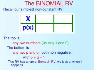
The BINOMIAL RV Recall our simplest non-constant RV: The top is any two numbers(usually 1 and 0) The bottom is any two p and q, both non negative, with p + q = 1 This RV has a name, Bernoulli RV, we look at when it happens.
Bernoulli Trials The Bernoulli RV happens whenever the experiment has just two possible outcomes. In fact, if the actual outcomes are not numerical we can make them so by calling one of them 1 and the other 0 (we could also use 17 or 347, but it gets cumbersome!) In everyday practice the two outcomes are called “success” (corresponding to 1) and “failure” (corresponding to 0). Careful …
The two words “success” and “failure” do not have to maintain their usual meaning, in some experiment success may mean the fish died, or the rocket exploded, or the baby was a female(I am being sexist, just for fun!) In our context • success simply means the outcome that corresponds to the value 1, and • failure means the outcome corresponding to the value 0. • The textbook calls them S and F(duh!)
Examples of Bernoulli Experiments Any experiment that has only two possible outcomes qualifies as a Bernoulli Experiment. The list is practically infinite. The hardest part is to decide what to call “success” and what to call “failure.” In the list to follow I am just having some fun. • Shoot an arrow at a target. Success means you miss (you keep the arrow) failure means you hit it. (You lose the arrow.) • Kiss a frog. Success means it turns into a prince(ss) failure means you turn into a frog.
Examples of Bernoulli Experiments (cont’d) • Take a penalty shot (soccer) Success means you score Failure means you don’t. (Note that if you are the goalie the point of view tends to reverse.) • Set your alarm for 6:00 am. Success means it wakes you up. Failure means you sleep till 11:00. • Submit to a drug test. Success means you test negative (never mind false negatives!) Failure means you test positive (never mind false positives!) You get the idea. Invent 5 more examples.
Bernoulli Trials Obviously a Bernoulli Experiment is a rather simple thing, just one of two outcomes. A “Bernoulli Trial” is a little more complex, but not that much. Essentially it is just a sequence of • n identical Bernoulli experiments (in each experiment the probability of success, and therefore of failure, is the same) • each individual experiment is independent of the others (we can multiply probabilities!) This second requirement is the hardest to verify, so most of the time we’ll just assume it is true. For example, in the penalty shot situation, you would expect the kicker to learn as she/he kicks, but we will assume they do not. The Binomial Random Variable is simply the number of successes in a Bernoulli Trial consisting of n Bernoulli experiments.
The Binomial Distribution Let’s try to build the probability distribution of the Binomial RV. For the sake of space we’ll take n = 10. So we are dealing with ten identical, independent Bernoulli experiments, and we are countingSuccesses. At least it’s easy to determine the range of our RV. It must be: 0, 1, 2, 3, 4, 5, 6, 7, 8, 9, 10 and the table looks like:
We have done the easy part, the top row. Now we go for the bottom row. Following my mother’s advice (a superb elementary school teacher) we take an even smaller number than 10, we take n = 5. We use the textbook’s notation of S and F. The simple outcome of five Bernoulli experiments is one of the following 32 outcomes (why 32?) SSSSS FSFSSFFSSFSSFFF SSSSFFFSSS FFSFS SFFFS SSSFSSFSSFFFFSSFFFFS SSFSS SFSFSFSFSFFFFSF SFSSS SFFSSFSFFSFFSFF FSSSS SSFSFFSSFFFSFFF FSSSFSSFFSSFFSFSFFFF FSSSF SSSFFSFFFSFFFFF F
For each of the 32 simple outcomes we count successes: SSSSS 5FSFSS3FFSSF2SSFFF2 SSSSF 4FFSSS 3FFSFS 2SFFFS2 SSSFS4SFSSF3FFFSS2FFFFS1 SSFSS 4SFSFS3FSFSF2FFFSF1 SFSSS 4SFFSS3FSFFS2FFSFF1 FSSSS 4SSFSF3FSSFF 2FSFFF1 FSSSF3SSFFS3SFFSF 2SFFFF1 FSSSF3SSSFF3SFFFS2FFFFF0
So in this case, assuming that p denotes the probability of success and 1 - p = q the probability of failure, and that p = q = 0.5 (this makes the 32 simple outcomes equally likely, it’s like tossing as fair coin) (count’em!)
First of all we take care of when p ≠ q Consider any simple outcome that has k successes, and therefore n-k failures, (think 3 successes and 2 failures) Since the experiments are independent we can multiply probabilities, therefore to that simple outcome we attach the probability pkq(n-k) Therefore to any outcome with 3 successes and 2 failures we attach the same probability. This says that p(3 successes) = (# outcomes with 3 S’s)x(p3q2) If we use k instead of 3 (and n-k instead of 2) we get:
p(k successes) = (# outcomes with k S’s)x(pkq(n-k)) All we have to do now is count how many simple outcomes have exactly k S’s Let’s get back to something simple, say 7 experiments.. The totality of simple outcomes is counted by observing that, in each of the boxes below we must put either S or F, and our choices multiply. So we get 27 = 128 simple outcomes.
Let’s see in how many ways we can get 4 successes in 7 Bernoulli experiments. Here are four S’s: S S S S Place them in the grid, one per box. Of course, what you have to do is chose four boxes, no repetition (one S per box) and order does not matter (any one S looks like any other.) Therefore the number of choices is ….
The Binomial RV, general formula Now we change 4 to k 7 to n and get that P(k successes in n indep., identical trials) = (# outcomes with k S’s)x(pkq(n-k)) =
Some important notation Observe that everything is known about a binomial RV (that is, range and probabilities) as soon as we know n and p. So we call THAT RV b(n,p) (b for binomial, duh) and the probability of k successes in THAT RV we denote by b(n,p,k) Therefore we have the formula
A final remark Computing a number like b(25,0.7,13) is no picnic, it boils down to But … , these numbers, being hard to find, have been tabulated, well, not quite, what the tables (on pp. 785 - 788) show is
In other words, what the tables show you (once you know n and p, and get to the appropriate table) is NOT b(n,p,k) BUT b(n,p,0) + b(n,p,1) + … +b(n,p,k-1)+b(n,p,k) So, if you need to compute b(20,0.7,15) You follow these steps • Find the appropriate table (p. 787, bottom) • Find the value in the table corresponding to 15 (call this UPT(15), it is • b(20,0.7,0) + … +b(20,0.7,15)) • Find UPT(14) and … • subtract. Now we do some examples on the board.
Normal Approximation to theBinomial Distribution Let X be b(n,p). We have learned that =E(X) = np and It turns out that, if the interval [0,n] contains
Then the two distributions B(n,p) and N( , ) are quite close to each other. Here = np and The condition about intervals boils down to: The figure in the next slide shows the “fit”
CAREFUL !! Suppose X is b(30,0.6) (as in the previous slide). How do we use the good “fit” to compute P(X = 20), or P(X > 15) or P(X ≤ 22) ? The procedure is simple but dangerous: Treat X as if it were , find the z values corresponding to the x values and use the normal tables. This is easier said than done.
The difficulty stems from the fact that the values of the binomial are individual integers, with their own probabilities, while the normal distribution attaches probabilities to intervals, not individual values. The way out, of course, is to think of each integer as the center of its own little sub-interval, one unit long. That is, for example, 20 is the center of the subinterval (19.5, 20.5), so to compute P(X=20) we proceed as follows:
We compute and from the formulas • We standardize (find the z-value) of 19.5 and 20.5 . We get 0.56 for 19.5 and 0.93 for 20.5. • We look at 0.93 and 0.56 in the normal tables and subtract. How about computing P(X > 17) ? Keep thinking in terms of subintervals. Clearly we want to catch (as integers) 18, 19, 20, …
So, in terms of those subintervals, we want to go from 17.5 on, that is we standardize 17.5 to get -0.19, and from the normal tables we get 0.5753, VOILA`. Now we compute P(15 < X ≤ 22) at the board, as well as P(15 ≤ X < 22), then you are on your own!