Download

1 / 11
120 likes | 338 Views
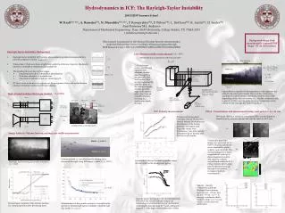
Understanding the Dynamics of Rayleigh-Taylor instabilities. Rayleigh-Taylor instabilities arise in fusion, super-novae, and other fundamental phenomena: start: heavy fluid above, light fluid below gravity drives the mixing process

E N D
Understanding the Dynamics of Rayleigh-Taylor instabilities • Rayleigh-Taylor instabilities arise in fusion, super-novae, and other fundamental phenomena: • start: heavy fluid above, light fluid below • gravity drives the mixing process • the mixing region lies between the upper envelope surface (red) and the lower envelope surface (blue) • 25 to 40 TB of data from simulations
1 2 3 4 5 6 7 8 9 10 20 30 40 We Provide the First Quantification of Known Stages of the Mixing Process mixing transition 1.0 (9524 bubbles) 0.5 0 linear growth -0.5 slope 1.536 Mode-Normalized Bubble Count(log scale) -1 0.1 Derivative of Bubble Count slope 1.949 -1.5 -2 strong turbulence slope 2.575 -2.5 Bubble Count 0.01 Derivative weak turbulence -3 t/(log scale)
We Provided the First Feature-Based Validation of a LES with Respect to a DNS LES (Large Eddy Simulation) Mode-Normalized Bubble Count DNS (Direct Numerical Simulation) Normalized Time
We Analyze High-Resolution Rayleigh–Taylor Instability Simulations maximum bubble • Large eddy simulation run onLinux cluster: 1152 x 1152 x 1152 • ~ 40 G / dump • 759 dumps, about 25 TB • Direct numerical simulation run on BlueGene/L: 3072 x 3072 x Z • Z depends on width of mixing layer • More than 40 TB • Bubble-like structures are observed in laboratory and simulations • Bubble dynamics are considered an important way to characterize the mixing process • Mixing rate = • There is no prevalent formal definition of bubbles
We Compute the Morse–Smale Complex of the Upper Envelope Surface Maximum F(x) = z F(x) on the surface is aligned against the direction of gravity which drives the flow Morse complex cells drawn in distinct colors In each Morse complex cell, all steepest ascending lines converge to one maximum
Saddle p1 p2 A Hierarchal Model is Generated by Simplification of Critical Points • Persistence is varied to annihilate pairs of critical points and produce coarser segmentations • Critical points with higher persistence are preserved at the coarser scales
The Segmentation Method is Robust From Early Mixing to Late Turbulence T=100 T=700 T=353
We Evaluated Our Quantitative Analysis at Multiple Scales Under-segmented Coarse scale Medium scale Number ofbubbles Over-segmented Timestep Fine scale
First Robust Bubble Tracking From Beginning to Late Turbulent Stages
1.0 (9524 bubbles) 0.5 0 -0.5 slope 1.536 Mode-Normalized Bubble Count(log scale) -1 0.1 Derivative of Bubble Count slope 1.949 -1.5 1 2 3 4 5 6 7 8 9 10 20 30 40 -2 slope 2.575 -2.5 Bubble Count 0.01 Derivative -3 t/(log scale) First Time Scientists Can Quantify Robustly Mixing Rates by Bubble Count