Download

1 / 79
800 likes | 908 Views
This study by Nick Bloom investigates the effects of uncertainty shocks on firms, using a structural model estimation and a simulation of the 9/11 event. The research analyzes stock market volatility, firm responses, and economic implications of increased uncertainty post-shocks.

E N D
The Impact of Uncertainty Shocks:Firm-Level Estimation and a 9/11 SimulationNick Bloom (Stanford & NBER)April 2007
Monthly US stock market volatility Black Monday* 9/11 Enron Russia & LTCM Franklin National Cambodia,Kent State Gulf War II Monetary turning point JFK assassinated OPEC I Asian Crisis Afghanistan Cuban missile crisis Gulf War I OPEC II Vietnam build-up Annualized standard deviation (%) Actual Volatility Implied Volatility Note: CBOE VXO index of % implied volatility, on a hypothetical at the money S&P100 option 30 days to expiry, from 1986 to 2004. Pre 1986 the VXO index is unavailable, so actual monthly returns volatilities calculated as the monthly standard-deviation of the daily S&P500 index normalized to the same mean and variance as the VXO index when they overlap (1986-2004). Actual and implied volatility correlated at 0.874. The market was closed for 4 days after 9/11, with implied volatility levels for these 4 days interpolated using the European VX1 index, generating an average volatility of 58.2 for 9/11 until 9/14 inclusive. * For scaling purposes the monthly VOX was capped at 50 affecting the Black Monday month. Un-capped value for the Black Monday month is 58.2.
Stock market volatility appears to proxy uncertainty • Political uncertainty correlated with stock market volatility(Mei & Guo 2002, Voth 2002, Wolfers and Zitewitz, 2006) • Professional forecaster spread over GDP growth correlated 0.437 with stock market volatility (bi-annual, Livingstone) • Cross-sectional industry TFP growth spread correlated 0.429 with stock market volatility (annual, NBER) • Common factor of exchange rate, oil price and interest rate volatility correlated 0.423 with stock market vol. (monthly)
Monthly stock market levels September 114 JFK assassinated Russian & LTCMDefault Vietnam build up Cuban missile crisis Asian Crisis Cambodia, Kent State Monetary cycle turning point WorldCom & Enron OPEC I, Arab-Israeli War Black Monday3 Gulf War II Gulf War I Franklin National financial crisis Afghanistan OPEC II Note: S&P500 monthly index from 1986 to 1962. Real de-trended by deflating by monthly “All urban consumers” price index, converting to logs, removing the time trend, and converting back into levels. The coefficient (s.e.) on years is 0.070 (0.002), implying a real average trend growth rate of 7.0% over the period.
The FOMC discussed uncertainty a lot after 9/11 Frequency of word “uncertain” in FOMC minutes 9/11 2001 2002 Source: [count of “uncertain”/count all words] in minutes posted on http://www.federalreserve.gov/fomc/previouscalendars.htm#2001
The FOMC also believed uncertainty mattered “The events of September 11 produced a marked increase in uncertainty ….depressing investment by fostering an increasingly widespread wait-and-see attitude about undertaking new investment expenditures”FOMC minutes, October 2nd 2001 “Because the attack significantly heightened uncertainty it appears that some households and some business would enter a wait-and-see mode….They are putting capital spending plans on hold”FOMC member Michael Moskow, November 27th
Motivation • Major shocks have 1stand 2nd moments effects • Policymakers believe both matter – is this right? • Lots of work on 1st moment shocks • Much less work on 2nd moment shocks • Closest work probably Bernanke (1983, QJE) • Predicts wave like effect of uncertainty flucatuations • I confirm, quantify & estimate this work
Summary of the paper Stage 1: Build and estimate structural model of the firm • Standard model augmented with • time varying uncertainty • mix of labor and capital adjustment costs • Estimate on firm data by Simulated Method of Moments Stage 2: Simulate stylized 2nd moment shock (micro to macro) • Generates rapid drop & rebound in • Hiring, investment & productivity growth • Confirm robustness to GE, risk-aversion, and AC estimates Stage 3: Compare to empirical evidence, and show reasonable fit • VAR results show volatility shocks cause a rapid drop and rebound in output (and employment) • 9/11 event study shows drop & rebound against expectations, plus a drop and rebound in cross-sectional investment activity
Time out… Two things that I tried to do: • Start with some kind of big picture, and also use a graph • Provide a summary of where I am going and what the results will be This risks are this is quite long – sometimes this can take while to talk through. If lots of early questions come up take some of them but also be discplined and simply move on
Model Estimation Results Shock Simulations
Firm Model outline Net revenue function, R Model has 3 main components Labor & capital “adjustment costs”, C Stochastic processes, E[ ] Firms problem = max E[ Σt(Rt–Ct) / (1+r)t ]
Time out… I put the previous slide in just to settle people down – it is obvious to most people (hence need to be fast) but useful as a guide.
Revenue function (1) Cobb-Douglas Production A is productivity, K is capital L is # workers, H is hours, α+β≤1 Constant-Elasticity Demand B is the demand shifter Gross Revenue Yis “demand conditions”, where Y1-a-b=A(1-1/e)B a=α(1-1/e), b=β(1-1/e)
Revenue function (2) Firms can freely adjust hours but pay an over/under time premium W1 and w2 chosen so hourly wage rate is lowest at a 40 hour week Net Revenue = Gross Revenue - Wages
“Adjustment costs” (1) Active literature with range of approaches, e.g. Look at convex & non-convex adjustment costs for both labor and capital 1 Convex typically quadratic adjustment costs 2 Non-convex typically fixed cost or partial irreversibility
Time out… The prior slide is controversial in some places (there is a lot of work in this area and not everyone agrees). So in advance of any important presentation: • Workout who will be your audience. Spend time looking at each persons page on the web-site – for a typical seminar this takes me about 3 or 4 hours (and I will already know some of the people as well) • Use this to make sure your presentation is correctly styled
“Adjustment costs” (2) • 1 period (month) time to build • Exogenous labor attrition rate δLand capital depreciation rate δK • Relative capital price is AR(1) stochastic
Stochastic processes – the “first moment” “Demand conditions” combines a macro and a firm random walk The macro process is common to all firms 1st MOMENT SHOCK The firm process is idiosyncratic Assumes firm and macro uncertainty move together - consistent with the data for large shocks (i.e. Campbell et al. 2001)
Stochastic processes – the “second moment” Uncertainty is AR(1) process with infrequent jumps 2nd MOMENT SHOCK • σσ=σ* so shocks roughly double average σ2t (note σZ is much smaller) • Prob(St=1) is 1/60, so one shock expected every 5 years
Time out… Be animated when explaining your work Also be enthusiastic – if you are not no-one else will be! Never self criticise your work – for example say (“this is very boring, only a nerd would do this” etc..)
The optimisation problem is tough Value function Simplify by solving out 1 state and 1 control variable • Homogenous degree 1 in (Y,K,L) so normalize by K • Hours are flexible so pre-optimize out Note: I is gross investment, E is gross hiring/firing and H is hours Simplified value function
Solving the model • Analytical methods for broad characterisation: • Unique value function exists • Value function is strictly increasing and continuous in (Y,K,L) • Optimal hiring, investment & hours choices are a.e. unique • Numerical methods for precise values for any parameter set
Example hiring/firing and investment thresholds Invest “Demand Conditions”/Capital: Ln(Y/K) Hire Inaction Fire “Real options” type effects Disinvest “Demand Conditions”/Labor: Ln(Y/L)
High and low uncertainty thresholds Larger “real options” at higher uncertainty Low uncertainty “Demand Conditions”/Capital: Ln(Y/K) High uncertainty “Demand Conditions”/Labor: Ln(Y/L)
Time out… Figures work well – these graphs are always much nicer to present then the theory and help get the message across Be creative in preparing your presentation and try to think how you can graphically display any complex results
Taking the model to real micro data • Model predicts many “lumps and bumps” in investment and hiring • See this in truly micro data – i.e. GMC bus engine replacement • But (partially) hidden in plant and firm data by cross-sectional and temporal aggregation • Address this by building cross-sectional and temporal aggregation into the simulation to consistently estimate on real data
Including cross-sectional aggregation • Assume firms owns large number of units (lines, plants or markets) • Units demand process combines macro, firm and unit shock where YF and YM are the firm and macro processes as before ΦU is relative unit uncertainty • Simplifying to solve following broad approach of Bertola & Caballero (1994), Caballero & Engel (1999), and Abel & Eberly (1999) • Assume unit-level optimization (managers optimize own “P&L”) • Links across units in same firm all due to common shocks
Including temporal aggregation • Shocks and decisions typically at higher frequency than annually • Limited survey evidence suggests monthly frequency most typical • Model at monthly underlying frequency and aggregate up to yearly
Model Estimation Results Shock Simulations
Estimation overview • Need to estimate all 20 parameters in the model • 8 Revenue Function parameters • production, elasticity, wage-functions, discount, depreciation and quit rates • 6 “Adjustment Cost” parameters • labor and capital quadratic, partial irreversibility and fixed costs • 6 Stochastic Process parameters • “demand conditions”, uncertainty and capital price process • No closed form so use Simulated Method of Moments (SMM) • In principle could estimate every parameter • But computational power restricts SMM parameter space • So (currently) estimate 6 adjustment cost parameters & pre-determine the rest from the data and literature
Simulated Method of Moments estimation • SMM minimizes distancebetween actual & simulated moments • Efficient W is inverse of variance-covariance of (ΨA - ΨS(Θ)) • Lee & Ingram (1989) show under the null W= (Ω(1+1/κ))-1 • Ω is VCV of ΨA, bootstrap estimated • κ simulated/actual data size, I use κ=10 actual data moments simulated moments weight matrix
Data is firm-level from Compustat • 10 year panel 1991 to 2000 to “out of sample” simulate 9/11 • Large continuing manufacturing firms (>500 employees, mean 4,500) • Focus on most aggregated firms • Minimize entry and exit • Final sample 579 firms with 5790 observations Note: This methodogly enables use of public firm data, avoiding the need to access the LRD, but relies on representativeness of public data see (Davis, Haltiwanger, Jarmin and Miranda, 2006)
Time out… Sad but true – for the job-market you need a little bit of algebra. Not loads, but a couple of slides somewhere with greek letters and curly deltas… If this really is inappropriate put it in the appendix – at least people flicking through your paper will see this
Model Estimation Results Shock Simulations
TABLE 2 “Adjustment cost” estimates Labor estimation moments Closer match between left and right columns of moments means a better fit Capital estimationmoments
Results for estimations on restricted models Capital “adjustment costs” only • Fit is only moderately worse • Both capital & labor moments reasonable • So capital ACs and pK dynamics approximate labor ACs Labor “adjustment costs” only • Labor moments fit is fine • Capital moments fit is bad (too volatile & low dynamics) • So OK for approximating labor data Quadratic “adjustment costs” only • Poor overall fit (too little skew and too much dynamics) • But industry and aggregate data little/no skew and more dynamics • So OK for approximating more aggregated data
Robustness - measurement error (ME) • Labor growth data contains substantial ME from • Combination full time, part-time and seasonal workers • Rounding of figures • First differencing to get ΔL/L • Need to correct in simulations to avoid bias • I estimate ME using a wage equation and find 11% • Hall (1989) estimates comparing IV & OLS & finds 8% • So I build 11% ME into main SMM estimators • Also robustness test without any ME and find larger FCL
Robustness – volatility measurement • Volatility process calibrated by share returns volatility • But could be concerns over excess volatility due to “noise” • Jung & Shiller (2002) suggest excess volatility more macro problem • Vuolteenaho (2002) finds “cash flow” drives 5/6 of S&P500 relative returns • Use 5/6 relative S&P500 returns variance and results robust • Find slightly higher adjustment costs
Time out… The last two slides I have typically do not present – I skip them having thought in advance they are less important
Model Estimation Results Shock Simulations
Simulating 2nd moment uncertainty shocks Run the thought experimentof just a second moment shock • Will add 1st moment shocks, but leave out initially for clarity To recap the uncertainty process is as follows Simulation of macro shock sets St=1 for one period (and Zt≡0) • σσ=σ*, so shocks doubles average σ2t (from initial graph) • Prob(St=1) is 1/60, so shocks every 5 years (from initial graph)
Simulation uncertainty macro “impulse” uncertainty shock Run model monthly with 100,000 firms for 5 years to get steady state then hit with uncertainty shock Uncertainty (σt) Month
Aggregate net hiring rate (%) uncertainty shock Net hiring rate Month Percentiles of firm net hiring rates (%) 99th Percentile Net hiring rate 95th Percentile 5th Percentile 1st Percentile Month
Macro gross investment rate (%) uncertainty shock Investment rate Month Firm percentiles of gross investment rates (%) 99th Percentile Investment rate 95th Percentile 5th Percentile 1st Percentile Month
Productivity growth rate (%) uncertainty shock Total Between Productivity growth Within Cross Month Productivity & hiring,period before shock Productivity & hiring,period after shock Gross hiring rate Gross hiring rate Productivity (logs) Productivity (logs)
GDP loss from uncertainty shock Estimate very rough magnitude of GDP loss, noting • Only from temporary 2nd moment shock (no 1st moment effects) • Ignores GE (will discuss shortly) so only look at first few months Rough GDP loss from an uncertainty shock (% of annual value) Reasonable size – uncertainty effects wipes out growth for ½ half year
Highlights importance identifying 1st & 2nd moment components of shocks Investment rate After a 1st moment shock expect standard U-shape downturn, bottoming out after about 6-18 monthsAfter a 2nd moment shock everything drops – just like a 1st moment shock- but then bounces back within 1 monthTo distinguish try using:(i) volatility indicators; (ii) plant spread;to help distinguish Hiring rate Prod. growth Month
Robustness – Risk aversion • Earlier results assumed firms risk-neutrality • Re-simulate with an “ad-hoc” risk correction where rt = a + bσt • Calibrated so that increases average (r) by 2.5% uncertainty shock risk-neutral Investment rate risk-averse Month
Robustness – Adjustment costs estimation • Need some non-convex costs - nothing with convex ACs only • Robust to type non-convex ACs (Dixit (1993) and Abel & Eberly (1996) show thresholds infinite derivate AC at AC≈0 ) PI=10%, all other AC=0 Aggregate Hiring Hiring Distribution Productivity FC=1%, all other AC=0 Aggregate Hiring Hiring Distribution Productivity