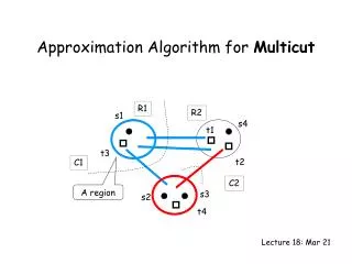
Introduction to Approximation Algorithms - Enhancing Problem-solving Efficiency
Learn about approximation algorithms and how they provide feasible solutions close to the optimal solution, reducing the time needed for solving complex problems efficiently. Discover heuristic methods, approximation ratios, and practical examples like the convex hull problem. Understand the significance of approximation algorithms in various scenarios, from convex hull computations to the traveling salesperson problem. Delve into algorithmic strategies like divide and conquer, Graham scan, and more. Explore the necessity and benefits of approximation algorithms in overcoming NP-hard problems efficiently.

Introduction to Approximation Algorithms - Enhancing Problem-solving Efficiency
E N D
Presentation Transcript
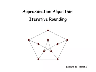
Approximation Algorithm Chapter 9
9-0 Approximation Algorithm (Concept) • Up to now, the best algorithm for solving an NP-complete problem requires exponential timein the worst case. It is too time-consuming. • To reduce the time required for solving a problem, we can relax the problem, and obtain a feasible solution “close” to an optimal solution • Other approaches ? • Supercomputer • Parallel processing • Distributed processing (Cryptography, Cryptanalysis)
9-0 Approximation Algorithm (Concept) • Why?we must use approximation algorithms. • 假設有一問題P, 至目前為止, 解決P的方法(找到Optimal Solution)至少為O(2n) Steps. 若目前有一最好Computer每秒可運算1 Step, 則試問該Computer要花多少時間來找到P的最佳解? • 一年有60*60*24*365=31536000秒, 故該Computer每年至多可計算31536000 Steps. • 若n = 1000, 則該Computer最快在(21000/ 31536000) 3*10292年才可找到P的最佳解. • 故若找到該問題的Optimal solution, 則目前全世界的人均看不到該結果了.
9-0 Approximation Algorithm (Concept) • Heuristic Methods. (啟發式,Educated guess) • 利用polynomial time algorithm (O(n2) steps), 找到一個解, 其解並不一定Optimal. • 若用該algorithm, 則只需102/ 31536000 0.033年即可找到一個feasible solution. • Heuristic algorithms是polynomial time algorithms, 其找到的答案可能非optimal solution. That is, heuristic algorithms do not guarantee optimal solutions. • How do we estimate our heuristic algorithm? • 作實驗or 模擬, 以比較方法的優劣 • 證明the output of heuristic algorithm與optimal solution的比率. 即證明我們的heuristic algorithm之輸出值與最佳解是很接近的. (Approximation Algorithms)
9-0 Approximation Algorithm (Concept) • Approximation Algorithms. • 若有一Approximation polynomial time algorithm (O(n2) steps) for the maximum problem, 找到一個解P(n), 而Optimal Solution為OPT. • 證明P(n)/OPT 2. • 2即是ratio of approximation to optimal. • Ratio的意義? (Dependent on Problem)
9-1 An approximation algorithm for convex hulls (Easy example to learn principle) • A convex hull of n points in the plane can be computed in O(nlogn) time in the worst case. • Recall: Chap 4.3 Divide and Conquer • Time complexity: T(n) = 2T(n/2) + O(n) = O(n log n)
Recall: 4-3 The convex hull problem • The divide-and-conquer strategy to solve the problem:
9-1 An approximation algorithm for convex hulls (cont.) • An approximation algorithm: • Step1:Find the leftmost and rightmost points.
9-1 An approximation algorithm for convex hulls (cont.) • Step2: Divide the points into K strips. Find the highest and lowest points in each strip.
9-1 An approximation algorithm for convex hulls (cont.) • Step3:Apply the Graham scan to those highest and lowest points to construct an approximate convex hull. (The highest and lowest points are already sorted by their x-coordinates.: Note Step 1 )
9-1 Algorithm 9-1 An approximation Algorithm for Convex Hull. • Input: A set of n points. • Output: An approximate convex hull of S. • Step 1: Find the leftmost and right most points of S, denoted as A1 and A2, respectively. (with minimum and maximum x-coordinates respectively). • Step 2: Divide the area bounded by A1 and A2 into k equally spaced strips and for each strip, select the points with the minimum and maximum y-coordinates. Denote the set of points selected in this step together with A1 and A2 as set P.
Algorithm 9-1 An approximation Algorithm for Convex Hull.(cont.) • Step 3: Construct the convex hull of P and use that as the approximate convex hull of S. • Time complexity: O(n+k) = O(n) Step 1: O(n) Step 2: O(n) Step 3: O(k) • Discussion: K is large • A feasible solution “close” to an optimal solution • Requiring more time
9-1 How good is the solution ? • How far away the points outside are from the approximate convex hull? L/K. (Why ?) • L: the distance between the leftmost and rightmost points.
Recall: 6-4 The 1-center problem • Given n planar points, find a smallest circle to cover these n points. • Thinking: Straightforward-method? • Selected any two points (?) or three points from n points Fig. 6-16 The 1-Center Problem
Thinking: Another simple problem • The constrained 1-center problem • Prune and search • Easy version: constrained 1-center problem • The center is restricted to lying on a straight line. • Time complexity: T(n)=T(3/4n)+O(n) • The general 1-center problem • Prune and search based on constrained 1-center problem • T(n) = T(15n/16)+O(n) • Thinking: An approximation Algorithm for 1-center problem
9-2 An approximation algorithm for Euclidean traveling salesperson problem (ETSP) • The ETSP is to find a shortest closed path through a set S of n points in the plane. • The ETSP is NP-hard. • Euclidean=> triangular inequality, in a plane. • Recall: Previous algorithms • Chapter 8 NP-Complete problems(Ch 8.7) • NP-Complete problem reduction • Chapter 5 Branch and Bound (Ch 5.7) • Lower Bound (Reduced cost matrix) • Chapter 7 Dynamic programming (Ch 7.2) • Multi-Stage Graph (Describing All Possible Tours)
Recall: Overview of NP-Complete problem reduction • SAT 3-SAT • 3-SAT CN (Chromatic number decision) • CN Exact cover • Exact cover Sum of subsets • Sum of subsets Partition • Partition Bin packing • Bin packing VLSI discrete layout • -------------------------------------------------------- • SAT Clique decision problem • Clique decision problem Node cover decision problem • -------------------------------------------------------- • SAT Directed Hamiltonian cycle • Directed Hamiltonian cycle TSP • -------------------------------------------------------- • Refer to Sec. 11.3, Sec. 11.4 and its exercise of [Horowitz and Shani 1998] for the proofs of more NP-complete problems.
Recall Ch 5.7 99=96+3 Fig 5-26 A Branch-and-Bound Solution of a Traveling Salesperson Problem. Because 117<126
Recall: 7-2 TSP • Find the shortest path: 1, 4, 3, 2, 1 5+7+3+2=17 Fig. A Multi-Stage Graph Describing All Possible Tours of a Directed graph.
9-2 An approximation algorithm for Euclidean traveling salesperson problem (ETSP) • Recall: (Data structure) • An Eulerian cycle of a graph is a cycle in the graph in which every vertex is visited not necessarily once (At least once, maybe twice), and each edge appears exactly once. • A graph is called Eulerian if it has an Eulerian cycle. • Euler proved that a graph G is Eulerian iff G is connected and all vertices in G have even degrees. • A Hamiltonian cycle is a round trip path along n edges of G=(V,E) which visits every vertexonceand returns to its starting vertex. • Traveling salespersonoptimization (decision) problem: A tour of a directed graph G=(V, E) is a directedcycle that includes every vertex in V. The problem is to find a tour of minimum cost . Easy Hard
9-2 Approximation Algorithm for ETSP • Input: A set S of n points in the plane. (Complete graph ?) • Output:An approximate traveling salesperson tour of S. • Step 1: Find a minimal spanning tree T of S. • Step 2: Find a minimal Euclidean weightedmatchingM on the set of vertices ofodd degrees in T. Let G=M∪T. • Step 3: Find an Eulerian cycle of G and then traverse it to find a Hamiltonian cycle as an approximate tour of ETSP by bypassing all previously visited vertices.
9-2 Approximation Algorithm for ETSP • E.g. Step1: Find a minimal spanning treeT of S 3 1 1 3 1 1 2 2
9-2 Approximation Algorithm for ETSP • Step2:The number of points with odd degrees must be even. , even (where di denotes the degree of each vertices) Find a minimal Euclidean weighted matching M ) • In order to construct an Eulerian graph, we must add some more edges to make all the vertices have even degrees to guarantee existing a Eulerian cycle.
9-2 Approximation Algorithm for ETSP • Step3: Find an Eulerian cycle of G and then traverse it to find a Hamiltonian cycle as an approximate tour of ETSP by bypassing all previously visited vertices. Bypassing visited vertices
9-2 Approximation Algorithm for ETSP • Time complexity: O(n3) Step 1: O(nlogn) • Kruskal method (Ch 4.1 Greedy method) Step 2: O(n3) Step 3: O(n) • How close the approximate solution to an optimal solution?
9-2 How good is the solution ? • The approximate tour is within 3/2 of the optimal one. • Reasoning: a minimal spanning tree T of S L: optimal tour j1…i1j2…i2j3…i2m {i1,i2,…,i2m}: the set of odd degree vertices in T. 2 matchings: M1={[i1,i2],[i3,i4],…,[i2m-1,i2m]} M2={[i2,i3],[i4,i5],…,[i2m,i1]} length(L) length(M1) + length(M2) (triangular inequality) 2 length(M ) length(M) 1/2 length(L ) G = T∪M length(T) + length(M) length(L) + 1/2 length(L) = 3/2 length(L) Two matching sets, Why? (From slide 22,23) Find M1, then generate another M2
9-3 An approximation algorithm for the bottleneck traveling salesperson problem • Minimize the longest edge of a tour. • This is a mini-max problem. • This problem is NP-complete. • The input data for this problem fulfill the following assumptions: • The graph is a complete graph. • All edges obey the triangular inequality rule • Bottleneck problem (Thinking an algorithm: Minimal Spanning Tree problem) • Mini-max problem • Max-mini problem
9-3 An algorithm for finding an optimal solution • Step1:Sort all edges in G = (V,E) into a non-decreasing sequence |e1||e2|…|em|. Let G(ei) denote the subgraph obtained from G by deleting all edges longer than ei. • Step2: i←1 • Step3: If thereexists a Hamiltonian cycle in G(ei), then this cycle is the solution and stop. • Step4: i←i+1 . Go to Step 3. This problem is also NP-complete
9-3 Approximation algorithm for BTSP • e.g. 6
9-3 Approximation algorithm for BTSP • There is a Hamiltonian cycle, A-B-D-C-E-F-G-A, in G(BD). • The optimal solution is 13. • Def : The t-th power of G=(V,E), denoted as Gt=(V,Et), is a graph that an edge (u,v)Et if there is a path from u to v with at most t edges in G. • If a graph G is bi-connected(See Next page =>Def) , then G2 has a Hamiltonian cycle.
9-3 Approximation algorithm for BTSP • E.g. bi-connected: For any two vertices, there are two disjoint path (No common vertex)
A E B D C A E B D C Articulation point “a” : Avertex “a” whose removal will split G into many parts. * B is an Art. Point • (u,v) s.t. every path between u and v contains “a”. A E B Remove node “A” D C Biconnected component A E Remove node “B” B D C Non-biconnected component
Biconnected Components(BC) • Undirected GraphG=(V,E) • G is biconnected if 2 vertex disjoint paths between each pair of vertices, or G has one edge. • G is biconnected iff it contains no articulation points. A E B D C
9-3 Approximation algorithm for BTSP • E.g. G is abi-connected graph
9-3 Approximation algorithm for BTSP • E.g. G2 of the Graph A Hamiltonian cycle A-B-C-D-E-F-G-A Fig. 9-14 G2 of the Graph in Fig 9-13.
Algorithm 9-3 An Approximation Algorithm to Solve the Bottleneck Traveling Salesperson Problem. • Input: A complete graph G=(V,E) where all edges satisfytriangular inequality. • Output: A tour in G whose longest edges isnot greater than twice of the value of an optimal solution to the special bottleneck traveling salesperson problem of G. • Step 1: Sort the edges into |e1||e2|…|em|. • Step 2: i := 1. • Step 3:If G(ei) is bi-connected, construct G(ei)2, find a Hamiltonian cycle in G(ei)2 and return this as the output, otherwise, go to Step 4. • Step 4: i := i + 1. Go to Step 3.
9-3 Approximation algorithm for BTSP (With equal to or less than edge-length:8)
9-3 Approximation algorithm for BTSP (With equal to or less than edge-length:9)
9-3 Approximation algorithm for BTSP • A Hamiltonian cycle: A-G-F-E-D-C-B-A. • the longest edge: 16 • Time complexity: polynomial time
9-3 Approximation algorithm for BTSP • The approximate solution is bounded by two times an optimal solution. • Reasoning: A Hamiltonian cycle is bi-connected. eop: the longest edge of an optimal solution G(ei): the first bi-connected graph |ei||eop| The length of the longest edge in G(ei)22|ei| (triangular inequality) 2|eop|
9-3 How good is the solution ? • If there is a polynomial approximation algorithm which produces a bound less than two, then NP=P. (The Hamiltonian cycle decision problem reduces to this problem.) • Proof: For an arbitrary graph G=(V,E), we expand G to a complete Gc: Cij = 1 if (i,j) E Cij = 2 if otherwise (The definition of Cij satisfies the triangular inequality.) Let V* denote the value of an optimal solution of the bottleneck TSP of Gc. V* = 1 G has a Hamiltonian cycle
9-3 How good is the solution ? • Because there are only two kinds of edges, 1 and 2 in Gc, if we can produce an approximate solution whose value is less than 2V*, then we can also solve the Hamiltonian cycle decision problem.
9.5 Recall: 3-7 partition bin packing • Bin packing problem • n items, each of size ci , ci > 0 bin capacity : C • Determine if we can assign the items into k bins, ci C , 1jk. ibinj E.g. {c1,c2,c3,c4}={1, 3, 7, 4}, B=2, C=8 Solution: first bin {1,7} and second bin {3, 4} <Theorem> partition bin packing.
9-5 An approximation algorithm for the bin packing problem • n items a1, a2, …, an, 0 ai 1, 1 i n, to determine the minimum number of bins of unit capacity to accommodate all n items. • E.g. n = 5, {0.3, 0.5, 0.8, 0.2 0.4} The bin packing problem is NP-hard. Fig. 9-27 An Example of the Bin-Packing Problem
9-5 An approximation algorithm for the bin packing problem • An approximation algorithm: (first-fit) place ai into the lowest-indexed bin which can accommodate ai. • S(ai): the size of ai • OPT(I): the size of bins for an optimal solution of an instance I • FF(I):the size of bins in the first-fit algorithm • C(Bi): the sum of the sizes of aj’s packed in bin Bi in the first-fit algorithm
9-5 An approximation algorithm for the bin packing problem • OPT(I) C(Bi) + C(Bi+1) 1 m non-empty bins: C(B1)+C(B2)+…+C(Bm) m/2 FF(I) = m <2 = 2 2 OPT(I) FF(I) < 2 OPT(I) The sum of any two bins must >1
9.6 The rectilinear m-center problem (Optional) • The sides of arectilinear square are parallel or perpendicular to the x-axis of the Euclidean plane. • The problem is to find m rectilinear squares covering all of the n given points such that the maximum side length of these squares is minimized. • This problem is NP-complete. • This problem for the solution with error ratio < 2 is also NP-complete. (See the example on the next page.)
9.6 The rectilinear m-center problem • Input: P={P1, P2, …, Pn} • The size of an optimal solution must be equal to one of the L ∞(Pi,Pj)’s, 1 i < j n, where L ∞((x1,y1),(x2,y2)) = max{|x1-x2|,|y1-y2|}.
9.6 The rectilinear m-center problem => An approximation algorithm • Input: A set P of n points, number of centers: m • Output: SQ[1], …, SQ[m]: A feasible solution of the rectilinear m-center problem with size less than or equal to twice of the size of an optimal solution. Step 1: Compute rectilinear distances of all pairs of two points and sort them together with 0 into an ascending sequence D[0]=0, D[1], …, D[n(n-1)/2]. Step 2: LEFT := 1, RIGHT := n(n-1)/2 //* Binary search Step 3: i := (LEFT + RIGHT)/2. Step 4: If Test(m, P, D[i]) is not “failure” then RIGHT := i-1 else LEFT := i+1 Step 5: If RIGHT = LEFT then return Test(m, P, D[RIGHT]) else go to Step 3.
9.6 The rectilinear m-center problem => Algorithm Test(m, P, r) • Input: point set: P, number of centers: m, size: r. • Output:“failure”, or SQ[1], …, SQ[m] m squares of size 2r covering P. Step 1: PS := P Step 2: For i := 1 to m do If PS then p := the point is PS with the smallest x-value SQ[i] := the square of size 2r with center at p PS := PS -{points covered by SQ[i]} else SQ[i] := SQ[i-1]. Step 3: If PS = then return SQ[1], …, SQ[m] else return “failure”. (See the example on the next page.)