Download
1 / 38
380 likes | 482 Views
Biostatistics in Practice. Session 3: Testing Hypotheses. Peter D. Christenson Biostatistician http://research.LABioMed.org/Biostat. Session 3 Preparation.

E N D
Biostatistics in Practice Session 3: Testing Hypotheses Peter D. Christenson Biostatistician http://research.LABioMed.org/Biostat
Session 3 Preparation We have been using a recent study on hyperactivity for the concepts in this course. The questions below based on this paper are intended to prepare you for session 3.
Session 3 Preparation 1. From Figures 1 and 2, we see that 153/209 = 73% of parents of the younger children and 144/160 = 90% of parents of the older children initially were interested but did not participate. Does it seem logical that the rate is lower for the 3-year-olds? Do you have any intuition on whether the magnitude of the 73% vs. 90% difference is enough to support an age difference, regardless of the logical reason?
Session 3 Preparation #1 153/209 144/160 73% ↔ Consented ↔ 90%
Session 3 Preparation #1 153/209 144/160 73% ↔ Consented ↔ 90% Not intuitive whether 73% vs. 90% is a “real” difference, i.e. reproducible or extrapolates to other persons.
Session 3 Preparation #1 153/209 144/160 73% ↔ Consented ↔ 90% Hypothesis testing compares 73% and 90%. It does not say how precise the %s are.
Session 3 Preparation • 2. Look at the left side of the bottom panel of Figure 3 and recall what we have said about confidence intervals. Would you conclude that there is a change in hyperactivity under Mix A? • 3. Repeat question 2 for placebo.
Session 3 Preparation: #2 and #3 Possible values for real effect. Zero is “ruled out”.
Session 3 Preparation 4. Do you think that the positive conclusion for question #3 has been "proven"? 5. Do you think that the negative conclusion for question #2 has been "proven"?
Session 3 Preparation 4. Do you think that the positive conclusion for question #3 has been "proven"? Yes, with 95% confidence. 5. Do you think that the negative conclusion for question #2 has been "proven"? No, since more subjects would give a narrower confidence interval. Hypothesis testing make a Yes or No conclusion whether there is an effect and quantifies the chances of a correct conclusion either way. Confidence intervals give possible magnitudes of effects.
Session 3 Goals Statistical testing concepts Three most common tests Software Equivalence of testing and confidence intervals False positive and false negative conclusions
Session 3 Data For this session, we will focus on another paper for which I have the raw data. Paper is posted on our class website. Subjects were hospitalized for many days, blood samples taken every 8 hours and vital signs recorded every hour. Subject is adrenal insufficient if 2 successive serum cortisols are low.
Goal: Do Groups Differ By More than is Expected By Chance? Cohan (2005) Crit Care Med;33:2358-66.
Goal: Do Groups Differ By More than is Expected By Chance? • First, need to: • Specify experimental units (Persons? Blood draws?). • Specify single outcome for each unit (e.g., Yes/No, mean or min of several measurements?). • Examine raw data, e.g., histogram, for meeting test requirements. • Specify group summary measure to be used (e.g., % or mean, median over units). • Choose particular statistical test for the outcome.
Outcome Type → Statistical Test WilcoxonTest Medians %s ChiSquareTest . . . Means t Test . . . Cohan (2005) Crit Care Med;33:2358-66.
Minimal MAP: Group Distributions of Individual Units Non-AI Group (N=38) Stem.Leaf # 7 79 2 7 00111234 8 6 5556777888 10 6 00112234 8 5 67999 5 5 3 1 4 79 2 4 04 2 ----+----+----+----+ Multiply Stem.Leaf by 10 AI Group (N=42) Stem.Leaf # 7 6 1 7 11334 5 6 555 3 6 01112344 8 5 5566778 7 5 01222234 8 4 57788 5 4 23 2 3 6 1 3 13 2 ----+----+----+----+ Multiply Stem.Leaf by 10 → Approximately normally distributed → Use means to summarize groups. → Use t-test to compare means.
Goal: Do Groups Differ By More than is Expected By Chance? • Next, need to: • Calculate a standardized quantity for the particular test, a “test statistic”. • Often: t=(Diff in Group Means)/SE(Diff) • Compare the test statistic to what it is expected to be if (populations represented by) groups do not differ. Often: t is approx’ly normal bell curve. • Declare groups to differ if test statistic is too deviant from expectations in (2) above. • Often: absolute value of t >~2.
t-Test for Minimal MAP: Step 1 • Calculate a standardized quantity for the particular test, a “test statistic”. Non AI N 38 Mean 63.4122807 Std Dev 8.7141575 SE(Mean) 1.41=8.71/√38 AI N 42 Mean 56.1666667 Std Dev 10.7824634 SE(Mean) 1.66=10.78/√42 Diff in Group Means = 63.4 - 56.2 = 7.2 (“Signal”) SE(Diff) ≈ sqrt[SEM12 + SEM22] = sqrt(1.662+1.412) ≈ 2.2 (“Noise”) Signal to Noise Ratio → Test Statistic = t = (7.2 - 0)/2.2 = 3.28
t-Test for Minimal MAP: Step 2 • Compare the test statistic to what it is expected to be if (populations represented by) groups do not differ. Often: t is approx’ly normal bell curve. Expected values for test statistic if groups do not differ. Area under sections of curve = probability of values in the interval. (0.5 for 0 to ∞) Prob (-2 to -1) is Area = 0.14 Expect Observed = 3.28 0.95 Chance
t-Test for Minimal MAP: Step 3 • Declare groups to differ if test statistic is too deviant. [How much?] Convention: “Too deviant” is < 5% chance → |t| >~2. “Two-tailed” = the 5% is allocated equally for either group to be superior. Expect 2.5% 2.5% Conclude: Groups differ since ≥3.28 has <5% if no difference in the entire populations. 95% Chance Observed = 3.28
t-Test for Minimal MAP: p value • Declare groups to differ if test statistic is too deviant. [How much?] p-value: Probability of a test statistic at least as deviant as observed, if populations really do not differ. Smaller values ↔ more evidence of group differences. p value = 2(0.0007) = 0.0014 <<0.05 Expect Area = 0.0007 Area = 0.0007 Observed = 3.28 95% Chance
t-Test: Technical Note • There are actually several types of t-tests: • Equal vs. unequal variance (variance =SD2), depending on whether the SDs are too different between the groups. [Yes, there is another statistical test for comparing the SDs.] Non AI N 38 Mean 63.4122807 Std Dev 8.7141575 SE(Mean) 1.41=8.71/√38 AI N 42 Mean 56.1666667 Std Dev 10.7824634 SE(Mean) 1.66=10.78/√42 SE(Diff) ≈ sqrt[SEM12 + SEM22] = sqrt(1.662+1.412) ≈ 2.2 is approximate. There are more complicated exact formulas that software implements.
t-Test: Another Note • There are other types of t-tests: • A two-sided t-test assumes that differences (between groups or pre-to-post) are possible in both directions, e.g., increase or decrease. • A one-sided t-test assumes that these differences can only be either an increase or decrease, or one group can only have higher or lower responses than the other group. This is very rare, and generally not acceptable.
Back to Paper: Normal Range SD = 8.7 SD = 10.8 N = 38 N = 42 What is the “normal” range for lowest MAP in AI patients, i.e., 95% of subjects were in approximately what range?
Back to Paper: Normal Range SD = 8.7 SD = 10.8 N = 38 N = 42 What is the “normal” range for lowest MAP in AI patients, i.e., 95% of subjects were in approximately what range? Answer: 56.2 ± 2(10.8) ≈ 35 to 78
Back to Paper: Confidence Intervals SD = 8.7 SD = 10.8 N = 38 N = 42 SE = 1.41 SE = 1.66 SE(Diff of Means) = 2.2 SE(Diff) ≈ sqrt of [SEM12 + SEM22] Δ= 63.4-56.2= 7.2 is the best guess for the MAP diff between the means of “all” AI and non-AI patients. We are 95% sure that diff is within ≈ 7.2±2SE(Diff) = 7.2±2(2.2) = 2.8 to 11.6.
Back to Paper: t-test Δ= 7.2 is statistically significant (p=0.0014); i.e., only 14 of 1000 sets of 80 patients would differ so much, if AI and non-AI really don’t differ in MAP. Is Δ= 7.2 clinically significant?
Confidence Intervals ↔ Tests Hyperactivity Paper p>0.05 p≈0.05 p<0.05
Confidence Intervals ↔ Tests The Algebra: |Δ/SE(Δ)| = |t| < 2 is equivalent to: |Δ| < 2 SE(Δ) is equivalent to: -2 SE(Δ) < Δ < 2 SE(Δ) is equivalent to: Δ - 2 SE(Δ) < 0 < Δ + 2 SE(Δ) Hypothesis Test Confidence Interval
Confidence Intervals ↔ Tests 95% Confidence Intervals Non-overlapping 95% confidence intervals, as here, are sufficient for significant (p<0.05) group differences. However, non-overlapping is not necessary. They can overlap and still groups can differ significantly.
Back to Paper: Experimental Units Cannot use t-test for comparing lab data for multiple blood draws per subject. bat least 100 g/kg/min of propofol administered at the time of blood draw, or any pentobarbital in the 48 hrs before the blood draw Generalization of t-test
Tests on Percentages Is 26.3% vs. 61.9% statistically significant (p<0.05), i.e., a difference too large to have a <5% of occurring by chance if groups do not really differ? Solution: Same theme as for means. Find a test statistic and compare to its expected values if groups do not differ. See next slide.
Tests on Percentages Cannot use t-test for comparing lab data for multiple blood draws per subject. Chi-Square Distribution Here, the signal in the test statistic is a squared quantity, expected to be 1. Area = 0.002 Expect Test statistic=10.2 >> 5.99, so p<0.05. In fact, p=0.002. 5.99 1 Observed = 10.2 95% Chance
Tests on Percentages: Chi-Square The chi-square test statistic (10.2 in the example) is found by first calculating what is the expected number of AI patients with MAP <60 and the same for non-AI patients, if AI and non-AI really do not differ for this. Then, chi-square is found as the sum of standardized (Observed – Expected)2. This should be close to 1, as in the graph on the previous slide, if groups do not differ. The value 10.2 seems too big to have happened by chance (probability=0.002) if there is no difference among “all” TBI subjects.
Back to t-Test Declare groups to differ if test statistic is too deviant. How much “deviance” is enough proof? Convention: “Too deviant” is < 5% chance → |t| >~2. Why not choose, say, |t|>3, so that our chances of being wrong are even less, <1%? Expect 2.5% 2.5% 95% Chance Observed = 3.28
Back to t-Test Convention: “Too deviant” is < 5% chance → |t| >~2. Why not choose, say, |t|>3, so that our chances of being wrong are even less, <1%? Expect <0.5% <0.5% >99% Chance Observed = 3.28 Answer: Then the chances of missing a real difference are increased, the converse wrong conclusion. This is analogous to setting the threshold for a diagnostic test of disease.
Power of a Study Statistical power is the sensitivity of a study to detect real effects, if they exist. It needs to be balanced with the likelihood of wrongly declaring effects when they are non-existent. Today, we have been keeping that error at <5%. Power is the topic for the next session #4.