Download

1 / 36
360 likes | 463 Views
Delve into determining a star’s distance, luminosity, and radius, unraveling the diverse types within the star family. Learn methods like trigonometric parallax and intrinsic brightness. Examine the Size (Radius) of Stars and the Hertzsprung-Russell Diagram, a tool to organize stars by luminosity and temperature. Explore luminosity classes and effects on spectral lines, understand binary stars, and the Center of Mass concept. Enhance your knowledge of stars and their unique properties in this informative chapter.

E N D
0 The Family of Stars Chapter 8:
0 We already know how to determine a star’s • surface temperature • chemical composition • surface density In this chapter, we will learn how we can determine its • distance • luminosity • radius • mass and how all the different types of stars make up the big family of stars.
0 Distances to Stars d in parsec (pc) p in arc seconds __ 1 d = p Trigonometric Parallax: Star appears slightly shifted from different positions of Earth on its orbit 1 pc = 3.26 LY The farther away the star is (larger d), the smaller the parallax angle p.
0 The Trigonometric Parallax Example: Nearest star, a Centauri, has a parallax of p = 0.76 arc seconds d = 1/p = 1.3 pc = 4.3 LY With ground-based telescopes, we can measure parallaxes p ≥ 0.02 arc sec => d ≤ 50 pc This method does not work for stars farther away than 50 pc.
0 Intrinsic Brightness / Absolute Visual Magnitude The more distant a light source is, the fainter it appears. The same amount of light falls onto a smaller area at distance 1 than at distance 2 => smaller apparent brightness. Area increases as square of distance => apparent brightness decreases as inverse of distance squared
0 Intrinsic Brightness / Absolute Visual Magnitude(II) The flux received from the light is proportional to its intrinsic brightness or luminosity (L) and inversely proportional to the square of the distance (d): L __ F ~ d2 Star A Star B Earth Both stars may appear equally bright, although star A is intrinsically much brighter than star B.
0 Distance and Intrinsic Brightness Example: Recall: Betelgeuse App. Magn. mV = 0.41 Rigel App. Magn. mV = 0.14 For a magnitude difference of 0.41 – 0.14 = 0.27, we find an intensity ratio of (2.512)0.27 = 1.28
0 Distance and Intrinsic Brightness Rigel appears 1.28 times brighter than Betelgeuse, Betelgeuse But Rigel is 1.6 times further away than Betelgeuse Thus, Rigel is actually (intrinsically) 1.28*(1.6)2 = 3.3 times brighter than Betelgeuse. Rigel
0 Absolute Visual Magnitude To characterize a star’s intrinsic brightness, define absolute visual magnitude (MV): Apparent visual magnitude that a star would have if it were at a distance of 10 pc.
0 Absolute Visual Magnitude(II) Back to our example of Betelgeuse and Rigel: Betelgeuse Rigel Difference in absolute magnitudes: 6.8 – 5.5 = 1.3 => Luminosity ratio = (2.512)1.3 = 3.3
0 The Distance Modulus If we know a star’s absolute magnitude, we can infer its distance by comparing absolute and apparent magnitudes: Distance Modulus = mV – MV = -5 + 5 log10(d [pc]) Distance in units of parsec Equivalent: d = 10(mV – MV + 5)/5 pc
0 The Size (Radius) of a Star We already know: flux increases with surface temperature (~ T4); hotter stars are brighter. But brightness also increases with size: Star B will be brighter than star A. A B Absolute brightness is proportional to radius squared, L ~ R2. Quantitatively: L = 4 p R2s T4 Surface flux due to a blackbody spectrum Surface area of the star
0 Example: Polaris has just about the same spectral type (and thus surface temperature) as our sun, but it is 10,000 times brighter than our sun. Thus, Polaris is 100 times larger than the sun. This causes its luminosity to be 1002 = 10,000 times more than our sun’s.
0 Organizing the Family of Stars: The Hertzsprung-Russell Diagram We know: Stars have different temperatures, different luminosities, and different sizes. To bring some order into that zoo of different types of stars: organize them in a diagram of Luminosity versus Temperature (or spectral type) Absolute mag. Hertzsprung-Russell Diagram Luminosity or Temperature Spectral type: O B A F G K M
The Hertzsprung Russell Diagram 0 Most stars are found along the mainsequence
The Hertzsprung-Russell Diagram (II) 0 Same temperature, but much brighter than MS stars Must be much larger Stars spend most of their active life time on the Main Sequence. Giant Stars Same temp., but fainter → Dwarfs
0 Radii of Stars in the Hertzsprung-Russell Diagram Rigel Betelgeuse 10,000 times the sun’s radius Polaris 100 times the sun’s radius Sun As large as the sun 100 times smaller than the sun
0 Luminosity Classes Ia Bright Supergiants Ia Ib Ib Supergiants II II Bright Giants III III Giants IV Subgiants IV V V Main-Sequence Stars
0 Luminosity effects on the width of spectral lines Same spectral type, but different luminosity • Lower gravity near the surfaces of giants • smaller pressure • smaller effect of pressure broadening • narrower lines
0 Examples: • Our Sun: G2 star on the main sequence: G2V • Polaris: G2 star with supergiant luminosity: G2Ib
0 Binary Stars More than 50% of all stars in our Milky Way are not single stars, but belong to binaries: Pairs or multiple systems of stars which orbit their common center of mass. If we can measure and understand their orbital motion, we can estimate the stellar masses.
0 The Center of Mass center of mass = balance point of the system. Both masses equal => center of mass is in the middle, rA = rB. The more unequal the masses are, the more it shifts toward the more massive star.
0 Estimating Stellar Masses Recall Kepler’s 3rd Law: Py2 = aAU3 Valid for the solar system: star with 1 solar mass in the center. We find almost the same law for binary stars with masses MA and MB different from 1 solar mass: aAU3 ____ MA + MB = Py2 (MA and MB in units of solar masses)
0 Examples: a) Binary system with period of P = 32 years and separation of a = 16 AU: 163 ____ MA + MB = = 4 solar masses. 322 b) Any binary system with a combination of period P and separation a that obeys Kepler’s 3. Law must have a total mass of 1 solar mass.
0 Visual Binaries The ideal case: Both stars can be seen directly, and their separation and relative motion can be followed directly.
0 Spectroscopic Binaries Usually, binary separation a can not be measured directly because the stars are too close to each other. A limit on the separation and thus the masses can be inferred in the most common case: Spectroscopic Binaries:
0 Spectroscopic Binaries (II) The approaching star produces blueshifted lines; the receding star produces redshifted lines in the spectrum. Doppler shift Measurement of radial velocities Estimate of separation a Estimate of masses
Spectroscopic Binaries (III) 0 Typical sequence of spectra from a spectroscopic binary system Time
0 Eclipsing Binaries Usually, inclination angle of binary systems is unknown uncertainty in mass estimates. Special case: Eclipsing Binaries Here, we know that we are looking at the system edge-on!
Eclipsing Binaries (II) 0 Peculiar “double-dip” light curve Example: VW Cephei
0 Eclipsing Binaries (III) Example: Algol in the constellation of Perseus From the light curve of Algol, we can infer that the system contains two stars of very different surface temperature, orbiting in a slightly inclined plane.
Masses of Stars in the Hertzsprung-Russell Diagram 0 Masses in units of solar masses The higher a star’s mass, the more luminous (brighter) it is: High masses L ~ M3.5 High-mass stars have much shorter lives than low-mass stars: Mass tlife ~ M-2.5 Low masses Sun: ~ 10 billion yr. 10 Msun: ~ 30 million yr. 0.1 Msun: ~ 3 trillion yr.
The Mass-Luminosity Relation 0 More massive stars are more luminous. L ~ M3.5
0 Surveys of Stars Ideal situation: Determine properties of all stars within a certain volume. Problem: Fainter stars are hard to observe; we might be biased towards the more luminous stars.
0 A Census of the Stars Faint, red dwarfs (low mass) are the most common stars. Bright, hot, blue main-sequence stars (high-mass) are very rare. Giants and supergiants are extremely rare.