Download

1 / 17
170 likes | 475 Views
Hybrid automata. Rafael Wisniewski Automation and Control, Dept. of Electronic Systems Aalborg University, Denmark. Hybrid Systems October 9th 2009. Why are we here?.

E N D
Hybrid automata Rafael Wisniewski Automation and Control, Dept. of Electronic Systems Aalborg University, Denmark Hybrid Systems October 9th 2009
Why are we here? "Control Engineers will have to master computer and software technologies to be able to build the systems of the future, and software engineers need to use control concepts to master ever-increasing complexity of computing systems.” (IFAC Newsletter December 2005 No.6)
Hybrid System A dynamical system with a non-trivial interaction of discrete and continuous dynamics • autonomous • switches • jumps • controlled • switches • jump • between manifolds • (Branicky 1995)
Hybrid Systems in Control(take up of CS ideas 1990 - …) • Hybrid Automata is the Spec. Language • Tools for simulation and model checking (Henzinger,Alur,Maler,Dang, …) • Bisimulation as abstraction technique (Pappas,Neruda,Koo, …) • Industrial Applications
Hybrid Automaton - Syntax . X = {x1, … xn} - variables, X dotted variables, X’ - primed variables (V, E) – control graph init: V preds(X) inv: V preds(X) flow: V preds(X X) jump: E preds(X X´) event: E . x´ = x-1
Labelled Transition System Q –states, e.g. (v=”Off”,x = 17.5) Q0– initial states, Q0 Q A –labels – transition relation, Q A Q
{ (v,x) – (v,x’) | R0and f: (0,) Rn s.t. f is diff. and f(0) = x and f() = x’ and flow(v)[X := f(t), X:= f(t)], t (0,)} . . Transition Semantics of HA X = {x1, … xn} - variables (V, E) – control graph init: V pred(X) inv: V pred(X) flow: V pred(X X) jump: E pred(X X’) event: E x´ = x . Q - states – {(v,x) | v V and inv(v)[X := x]} Q0– initial states - {(v,x) Q | init(v)[X := x]} A - labels - R0 { (v,x) – (v’,x’) | e E(v,v’)and event(e) = and jump(e) [X:= x, X’:=x’]}
Computation tree: = q00 a q10 q11 ... q1n1 … q200 q201 q210 q211 q13 Tree Semantics Q - states, {(v,x) | v V and inv(v)[X := x]} Q0– initial states, … A - labels, … - transition relation, Q A Q
Trace Semantics Q - states, {(v,x) | v V and inv(v)[X := x]} Q0– initial states, … A - labels R0 - transition relation, Q A Q Trajectory: = <(a0,q0)…(ai,qi)…> where q0 Q0 and qi–aiqi+1, i 0 • Live Transition System: (S, L = { | infinite from S}) • Machine Closed: finite from S, prefix(L) • Duration of is sum of time labels. • S is non-Zeno: duration of L diverges, Machine closed • (ompare with the two tank example)
{ (v,x) – (v,x’) | R0and f: (0,) Rn s.t. f is diff. and f(0) = x and f() = x’ and flow(v)[X := f(t), X:= f(t)], t (0,)} . . Time Abstract Semantics X = {x1, … xn} - variables (V, E) – control graph init: V pred(X) inv: V pred(X) flow: V pred(X X) jump: E pred(X X’) event: E . Q - states – {(v,x) | v V and inv(v)[X := x]} Q0– initial states - {(v,x) Q | init(v)[X := x]} B - labels - {} - finite ! { (v,x) – (v’,x’) | e E(v,v’)and event(e) = and jump(e) [X := x]}
Composition of Transition Systems Q - states Q0– initial states, … A - labels, … - transition relation, Q A Q S = S1 || S2 with : A1 A2 A Composition of hybrid automata : Q = Q1 Q2 Q0 = Q10 Q20 (q1,q2) –a (q1’,q2’) iff (qi –ai qi’, i=1,2 and a = a1a2 is defined Remark p 7
X = {x1, … xn} - variables (V, E) – control graph init: V preds(X) inv: V preds(X) flow: V preds(X X) jump: E preds(X X’) event: E . Classes of Hybrid Automata . • Rectangular init, inv, flow (x Iflow), • jump (x = (x,y) I, x’ = (x’,y’), x’ I’ ,y’=y) • Singular – rectangular with Iflow a point • Timed – singular with Iflow = [1,1]n • Multirectangular …
Timed Automaton X = {x1, … xn} - variables (V, E) – control graph init: V pred(X) inv: V pred(X) flow: V pred(X X) jump: E pred(X X’) . Init(v): v = v0 and X = 0, where v0 V inv(v): X <= C , where C is rational flow(v): X = 1 jump(e) : A boolean combination of X <= C, X < C and Y = 0, where Y X’’ .
Trace Semantics Q - states – {(v,x) | v V and inv(v)[X := x]} Q0 – initial states - {(v,x) Q | init(v)[X := x]} B - labels - {} { (v,x) – (v’,x’) | e E(v,v’), event(e) = , jump(e) [X := x]} { (v,x) – (v,x’) | f(0) = x,f() = x’ , flow(v)[X := f(t), X:= f(t)], t (0,)} Trajectory: = <(a0,q0)…(ai,qi)…> where q0 Q0 and qi–aiqi+1, i 0
Symbolic Analysis Q - states Q0 – initial states, … A - labels, … - transition relation, A QQ a Theory: T = {p1, … pn … }, p is a predicate, e.g. pred(X V) Meaning of p: [p] Q q1 q2 iff p(q1) = p(q2) for all p T
Symbolic Bisimilarity Computation prea(R’) R’ R