Download

1 / 17
270 likes | 1.98k Views
Flow Measurement(basics). Ashvani Shukla C&I Reliance. INTRODUCTION.

E N D
Flow Measurement(basics) Ashvani Shukla C&I Reliance
INTRODUCTION • In the physical world, mechanical engineers are frequently required to monitor or control the flow of various fluids through pipes, ducts and assorted vessels. This fluid can range from thick oils to light gasses. While some techniques work better with some groups of fluids, and less well with others, some are not at all suitable for some applications. In this primer on fluid flow instrumentation we will look at a wide variety of flow transducers and their application in the physical world.
Fluid flow measurement • Fluid flow measurement can encompass a wide variety of fluids and applications. To meet this wide variety of applications the instrumentation industry has, over many years, developed a wide variety of instruments. The earliest known uses for flow come as early as the first recorded history. The ancient Sumerian cities of UR and Kish, near the Tigris and Euphrates rivers (around 5000 B.C.) used water flow measurement to manage the flow of water through the aqueducts feeding their cities. In this age the a simple obstruction was placed in the water flow, and by measuring the height of the water flowing over the top of the obstruction, these early engineers could determine how much water was flowing. In 1450 the Italian art architect Battista Alberti invented the first mechanical anemometer. It consisted of a disk placed perpendicular to the wind, and the force of the wind caused it to rotate. The angle of inclination of the disk would then indicate the wind velocity. This was the first recorded instrument to measure wind speed. An English inventor, Robert Hooke reinvented this device in 1709, along with the Mayan Indians around that same period of time. Today we would look down our noses at these crude methods of flow measurement, but as you will see, these crude methods are still in use today.
TYPE OF FLOW • There are in general three types of fluid flow in pipes • laminar • turbulent • transient • Laminar flow • Laminar flow generally happens when dealing with small pipes and low flow velocities. Laminar flow can be regarded as a series of liquid cylinders in the pipe, where the innermost parts flow the fastest, and the cylinder touching the pipe isn't moving at all. • Shear stress in a laminar flow depends almost only on viscosity - μ - and is independent of density - ρ. • Turbulent flow • In turbulent flow vortices, eddies and wakes make the flow unpredictable. Turbulent flow happens in general at high flow rates and with larger pipes. • Shear stress in a turbulent flow is a function of density - ρ. • Transitional flow
CONTINUE….. • Transitional flow is a mixture of laminar and turbulent flow, with turbulence in the center of the pipe, and laminar flow near the edges. Each of these flows behave in different manners in terms of their frictional energy loss while flowing and have different equations that predict their behavior. • Turbulent or laminar flow is determined by the dimensionless Reynolds Number. • Reynolds Number • The Reynolds number is important in analyzing any type of flow when there is substantial velocity gradient (i.e. shear.) It indicates the relative significance of the viscous effect compared to the inertia effect. The Reynolds number is proportional to inertial force divided by viscous force. • The flow is • laminar when Re < 2300 • transient when 2300 < Re < 4000 • turbulent when 4000 < Re
TYPE OF FLOW • Uniform Flow, Steady Flow • It is possible - and useful - to classify the type of flow which is being examined into small number of groups. If we look at a fluid flowing under normal circumstances - a river for example - the conditions at one point will vary from those at another point (e.g. different velocity) we have non-uniform flow. If the conditions at one point vary as time passes then we have unsteady flow. Under some circumstances the flow will not be as changeable as this. He following terms describe the states which are used to classify fluid flow: • • uniform flow: If the flow velocity is the same magnitude and direction at every point in the fluid it is said to be uniform. • • non-uniform: If at a given instant, the velocity is not the same at every point the flow is non-uniform. (In practice, by this definition, every fluid that flows near a solid boundary will be non-uniform - as the fluid at the boundary must take the speed of the boundary, usually zero. However if the size and shape of the of the cross-section of the stream of fluid is constant the flow is considered uniform.) • • steady: A steady flow is one in which the conditions (velocity, pressure and cross-section) may differ from point to point but DO NOT change with time. • unsteady: If at any point in the fluid, the conditions change with time, the flow is described as unsteady. (In practice there is always slight variations in velocity and pressure, but if the average values are constant, the flow is considered steady.
CONTINUOUS • Combining the above we can classify any flow in to one of four type: • 1. Steady uniform flow. Conditions do not change with position in the stream or with time. An example is the flow of water in a pipe of constant diameter at constant velocity. Fluid Mechanics Fluid Dynamics: The Momentum and Bernoulli Equations. • 2. Steady non-uniform flow. Conditions change from point to point in the stream but do not change with time. An example is flow in a tapering pipe with constant velocity at the inlet - velocity will change as you move along the length of the pipe toward the exit. • 3. Unsteady uniform flow. At a given instant in time the conditions at every point are the same, but will change with time. An example is a pipe of constant diameter connected to a pump pumping at a constant rate which is then switched off. • 4. Unsteady non-uniform flow. Every condition of the flow may change from point to point and with time at every point. For example waves in a channel.
CONTINUOUS • Compressible or Incompressible All fluids are compressible - even water - their density will change as pressure changes. Under steady conditions, and provided that the changes in pressure are small, it is usually possible to simplify analysis of the flow by assuming it is incompressible and has constant density. As you will appreciate, liquids are quite difficult to compress - so under most steady conditions they are treated as incompressible. In some unsteady conditions very high pressure differences can occur and it is necessary to take these into account - even for liquids. Gasses, on the contrary, are very easily compressed, it is essential in most cases to treat these as compressible, taking changes in pressure into account.
continuous • Three-dimensional flow Although in general all fluids flow three-dimensionally, with pressures and velocities and other flow properties varying in all directions, in many cases the greatest changes only occur in two directions or even only in one. In these cases changes in the other direction can be effectively ignored making analysis much more simple. Flow is one dimensional if the flow parameters (such as velocity, pressure, depth etc.) at a given instant in time only vary in the direction of flow and not across the cross-section. The flow may be unsteady, in this case the parameter vary in time but still not across the cross-section. An example of one-dimensional flow is the flow in a pipe. Note that since flow must be zero at the pipe wall - yet non-zero in the Centre - there is a difference of parameters across the cross-section. Should this be treated as two-dimensional flow? Possibly - but it is only necessary if very high accuracy is required. A correction factor is then usually applied.
continuous • Flow is two-dimensional if it can be assumed that the flow parameters vary in the direction of flow and in one direction at right angles to this direction. Streamlines in two-dimensional flow are curved lines on a plane and are the same on all parallel planes. An example is flow over a weir foe which typical streamlines can be seen in the figure below. Over the majority of the length of the weir the flow is the same - only at the two ends does it change slightly. Here correction factors may be applied. One dimensional flow
Flow rate. • Mass flow rate If we want to measure the rate at which water is flowing along a pipe. A very simple way of doing this is to catch all the water coming out of the pipe in a bucket over a fixed time period. Measuring the weight of the water in the bucket and dividing this by the time taken to collect this water gives a rate of accumulation of mass. This is know as the mass flow rate. • Volume flow rate - Discharge. More commonly we need to know the volume flow rate - this is more commonly know as discharge. (It is also commonly, but inaccurately, simply called flow rate). The symbol normally used for discharge is Q. The discharge is the volume of fluid flowing per unit time. Multiplying this by the density of the fluid gives us the mass flow rate.
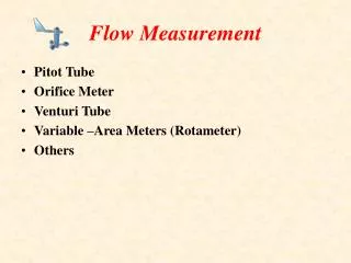
Type of flow measurement • The most common principals for fluid flow metering are: • Differential Pressure Flow meters • Velocity Flow meters • Positive Displacement Flow meters • Mass Flow meters • Open Channel Flow meters
1.Differential Pressure Flow meters • In a differential pressure drop device the flow is calculated by measuring the pressure drop over an obstructions inserted in the flow. The differential pressure flow meter is based on the Bernoulli's Equation, where the pressure drop and the further measured signal is a function of the square flow speed.
Common types of differential pressure flow meters are: • Orifice Plates • Flow Nozzles • Venturi Tubes • Variable Area - Rota meters • Orifice Plate An orifice plate is a device used for measuring flow rate, for reducing pressure or for restricting flow (in the latter two cases it is often called a restrictionplate). Either a volumetric or mass flow rate may be determined, depending on the calculation associated with the orifice plate.Withan orifice plate, the fluid flow is measured through the difference in pressure from the upstream side to the downstream side of a partially obstructed pipe. The plate obstructing the flow offers a precisely measured obstruction that narrows the pipe and forces the flowing fluid to constrict.
continuous • Orifice Plate is the heart of the Orifice Meter. It restricts the flow and develops the Differential Pressure which is proportional to the square of the flow rate. The flow measuring accuracy entirely depends upon the quality of Orifice plate, its installation and maintains. • When measuring wet gas or saturated steam a weep hole is drilled in a concentrically bored orifice plate. This is a small hole drilled on the orifice plate such that its location is exactly on ID of the main pipe.
Interesting, right? This is just a sneak preview of the full presentation. We hope you like it! To see the rest of it, just click here to view it in full on PowerShow.com. Then, if you’d like, you can also log in to PowerShow.com to download the entire presentation for free.