Introduction to Statistics and Data Analysis - Course Overview B01.1305
This course, B01.1305, provides a comprehensive introduction to statistics and data analysis. Led by Professor Balkin, students will explore statistical principles, types of data, and methods for univariate analysis using Minitab. Key topics include descriptive statistics, probability, statistical inference, and regression analysis. The semester emphasizes real-world applications, enabling students to enhance their business decision-making skills through effective data interpretation.

Introduction to Statistics and Data Analysis - Course Overview B01.1305
E N D
Presentation Transcript
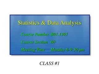
Statistics & Data Analysis Course Number B01.1305 Course Section 60 Meeting Time Monday 6-9:30 pm CLASS #1
Class #1 Outline • Introduction to the instructor • Introduction to the class • Review of syllabus • Introduction to statistics • Class Goals • Types of data • Graphical and numerical methods for univariate series • Minitab Tutorial
Professor Balkin’s Info • Ph.D. in Business Administration, Penn State • Masters in Statistics, Penn State • Mathematics/Economics and Music, Lafayette College • Employment • Pfizer Inc. • Management Science Group; Sept. 2001 – current • Ernst & Young • Quantitative Economics and Statistics Group; June 1999 – August 2001
What is Statistics? • STATISTICS: A body of principles and methods for extracting useful information from data, for assessing the reliability of that information, for measuring and managing risk, and for making decisions in the face of uncertainty. • POPULATION: set of measurements corresponding to the entire collection of units • SAMPLE: set of measurements that are collected from a population • OBJECTIVES: • To make inferences about a population from a sample, including the extent of uncertainty • Design the data collection process to facilitate drawing valid inferences
Reasons for Sampling • Typically due to prohibitive cost of contacting millions of people or performing costly experiments • Election polls query about 2,000 voters to make inferences regarding how all voters cast their ballots • Sometimes the sampling process is destructive • Sampling wine quality
Statistics in Everyday Life • Monthly Unemployment Rates (BLS) • Consumer Price Index • Presidential Approval Rating • Quality and Productivity Improvement • Scientific Inquiry • Training effectiveness • Advertising impact
Interesting Statistical Perspectives • “Statistical thinking will one day be as necessary for efficient citizenship as the ability to read and write”. • (H. G. Wells) • “There are three kinds of lies -- Lies, damn lies, and statistics”. • (Benjamin Disraeli) • “You’ve got to know when to hold ‘em, know when to fold ‘em.” • (Kenny Rogers, in The Gambler) • “The average U. S. household has 2.75 people in it.” • (U. S. Census Bureau, 1980) • “4 out of 5 dentists surveyed recommended Trident Sugarless Gum for their patients who chew gum.” • (Advertisement for Trident)
Semester Overview • Understanding data • Intro to descriptive statistics, interpreting data, and graphical methods • Dealing with and quantifying uncertainty • Random variables and probability • Using samples to make generalizations about populations • Assessing whether a change in data is beyond random variation • Modeling relationships and predicting • Using sample data to create models that give predictions for all values of a population
Goals for this Class • To gain an understanding of descriptive statistics, probability, statistical inference, and regression analysis so that it may be applied to your job • To be able to identify when statistical procedures are required to facilitate your business decision making • To be able to identify both good and poor use of statistics in business
Goals for Me • To teach you statistics and data analysis effectively • To improve my effectiveness as an instructor
My Promise To You • I will not teach you anything in this class that is not regularly used in business and industry • If you ask, “Where is this used?” I will have a real example for you
Example: Data Types • Business Horizons (1993) conducted a comprehensive survey of 800 CEOs who run the country's largest global corporations. Some of the variables measured are given below. Classify them as quantitative or qualitative. • State of birth • Age • Educational Level • Tenure with Firm • Total Compensation • Area of Expertise • Gender
CHAPTER 2 Summarizing Data about One Variable
Introduction • Unorganized mass of numbers is difficult to interpret • First task in understanding data is summarizing it • Graphically • Numerically
Chapter Goals • Distinguish between qualitative and quantitative variables • Learn graphic representations of univariate data • Learn numerical representations of univariate data • Investigate data acquired over time
Distribution of Values • Distribution is essentially how many times each possible data values occur in a set of data. • Methods for displaying distributions • Qualitative data • Frequency table • Bar charts • Quantitative data • Histograms • Stem-Leaf diagrams • Boxplots
Example: Qualitative Data • Background: A question on a market research survey asked 17 respondents the size of their households • Data: 1,1,1,2,2,2,2,2,3,3,3,3,3,3,4,4,6 • Frequency Table
Example: Qualitative Data (cont.) • Barchart: Plot of frequencies each category occurs in the data set
Example: Quantitative Data • Background: Forbes magazine published data on the best small firms in 1993. These were firms with annual sales of more than five and less than $350 million. Firms were ranked by five-year average return on investment. The data are the annual salary of the chief executive officer for the first 60 ranked firms. • Data (in thousands): 145 621 262 208 362 424 339 736 291 58 498 643 390 332 750 368 659 234 396 300 343 536 543 217 298 1103 406 254 862 204 206 250 21 298 350 800 726 370 536 291 808 543 149 350 242 198 213 296 317 482 155 802 200 282 573 388 250 396 572
Example: Quantitative Data (cont.) • Histograms are constructed in the same way as bar charts except: • User must create classes to count frequencies • Bars are adjacent instead of separated with space
Example: Quantitative Data (cont.) • Questions: • What is the typical value of CEO salary? • How much variability is there around this value? • What is the general shape of the data? • Histogram characteristics: • Central tendency • Variability • Skewness • Modality • Outliers
Example: Stem-Leaf Diagram • Background: Telecom company wants to analyze the time to complete new service orders measured in hours • Data: 42 21 46 69 87 29 34 59 81 97 64 60 87 81 69 77 75 47 73 82 91 74 70 65 86 87 67 69 49 57 55 68 74 66 81 90 75 82 37 94 • Diagram: 2 | 19 3 | 47 4 | 2679 5 | 579 6 | 045678999 7 | 0344557 8 | 111226777 9 | 0147
Measures of Central Tendency • Mode: Value or category that occurs most frequently • Median: Middle value when the data are sorted • Mean: Sum of measurements divided by the number of measurements
Example: Mode • Background: A question on a market research survey asked 17 respondents the size of their households • Data: 1,1,1,2,2,2,2,2,3,3,3,3,3,3,4,4,6 • Frequency Table Mode
Example: Median • Background: A question on a market research survey asked 17 respondents the size of their households • Data: 1,1,1,2,2,2,2,2,3,3,3,3,3,3,4,4,6 • Since the n=17 observations, • Median is the (n+1)/2 = 9th observation Median
Example: Mean • Background: Cable company wants to know how long an installer spends at each stop. One employee performed five installations in one day and recorded how many minutes she was at each location. • Data: 45, 23, 36, 29, 52 • Mean = (45+23+36+29+52) / 5 = 37 minutes
Example: Back to the CEO’s Salaries Mean = 404.1695 Median = 350 WHY THE DIFFERENCE?
Measures of Variation • A primary reason for using statistics is due to variability • If there was no variability, we would not nee statistics • Examples: • Worker productivity • Stock market • Promotional expenditures • Measures • Standard deviation: variation around the mean • Range: distance between smallest and largest observations
Standard Deviation • Standard Deviation: summarizes how far away from the mean the data value typically are. • Calculation • Find the deviations by subtracting the mean from each data value • Square these deviations, add them up, and divide by n-1 • Take the square root of this number
Example: Standard Deviation • Background: Your firm spends $19 Million per year on advertising, and management is wondering if that figure is appropriate. Other firms in your industry have a mean advertising expenditure of $22.3 Million per year.
Example: Standard Deviation (cont.) • Difference from peer group average is $3.3 Million • This difference is smaller than the industry standard deviation of $9.18 Million • Conclusion: You advertising budget, while slightly below the industry average, is typical compared with your industry peers
Empirical Rule • If the histogram for a given sample is unimodal and symmetric (mound-shaped), then the following rule-of-thumb may be applied: • Let represent the sample mean and s the sample standard deviation. Then
Example: Stock Market Volatility • Description: Stock market returns are supposed to be unpredictable. Let’s see if the empirical rule holds true • Data: S&P-500 Daily returns; Jan 01, 1998 – May 17, 2002 • Mean = 0.0002 • St. Dev. = 0.0128 • 72.8% (95.3%) of the returns fallbetween the sample mean plusand minus one (two) st.dev.
Inter-Quartile Range • Inter-Quartile Range (IQR) provides an alternative approach to measuring variability • Computation: • Sort the data and find the median • Divide the data into top and bottom halves • Find the median of both halves. These are the 25th and 75th percentiles • IQR = 75th percentile – 25th percentile • Outlier Measure – Any value outside the inner fences is an outlier candidate • Lower inner fence = 25th percentile – 1.5 IQR • Upper inner fence = 75th percentile + 1.5 IQR
Box-Plot – S&P-500 Example Data: S&P-500 Daily returns; Jan 01, 1998 – May 17, 2002 Upper inner fence Outliers 75th percentile Median 25th percentile Lower inner fence
Why Use Minitab??? • Goal of course is to learn statistical concepts • Most statistical analyses are performed using computers • Each company may use a different statistical package • YES…Minitab is used in business! • Typically in quality control and design of experiments • EXCEL has very limited statistical functionality and is considerably more difficult to use than Minitab • There are many stat packages (SAS, SPSS, Systat, Splus, R, Statistica, Mathematica, etc.) • Minitab is the easiest program to use right away • Excellent Help facilities • Statistical glossary built-in
Minitab Tutorial – Case Study 1 • A hotel kept records over time of the reasons why guest requested room changes. The frequencies were as follows • Room not clean 2 • Plumbing not working 1 • Wrong type of bed 13 • Noisy location 4 • Wanted nonsmoking 18 • Didn’t like view 1 • Not properly equipped 8 • Other 6
Minitab Tutorial – Case Study 2 • Exercise 2.8 in book • Produce graphics • Produce descriptive statistics
Minitab Tutorial – Case Study 3 • Diversification??? • Data: S&P-500 and IBM daily returns from Jan 01, 1998 through May 17, 2002
Next Time • Probability and Probability Distributions