Download
1 / 40
400 likes | 569 Views
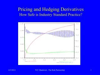
Pricing and Hedging Derivatives How Safe is Industry Standard Practice?. Pricing and Hedging Options How Safe is Industry Standard Practice?. • Prices are often seriously wrong

E N D
Pricing and Hedging DerivativesHow Safe is Industry Standard Practice? W.F. Shadwick , The Risk Partnership
Pricing and Hedging OptionsHow Safe is Industry Standard Practice? • Prices are often seriously wrong • Sensitivities are rendered meaningless either by inadequate computational technology or, even worse, flawed financial modelling. • Both of these problems are exacerbated by attempts to incorporate ‘improved’ treatments of volatility The implications of this are serious given the rapid growth of OTC derivatives and the increased scrutiny arising from FAS133 and similar new requirements. W.F. Shadwick , The Risk Partnership
What is this view based on? • Experience with a variety of systems in widespread use • Extensive anecdotal evidence • But probably the most convincing basis is the historical record W.F. Shadwick , The Risk Partnership
The Evidence provided by 1) The contrast between what good engineering practice should have produced in the 30 years since Black Scholes and Merton and what actually happened 2) The features of current practice which resulted from the failure to meet basic engineering standards W.F. Shadwick , The Risk Partnership
What should we expect from models? • Mathematical models, in any field, are our best attempt to predict the future from the data we have at present • They always fail at some level–even in the exact sciences • Financial models have to be used with this in mind but the same discipline which optimises their effectiveness in science and engineering is also required in finance. W.F. Shadwick , The Risk Partnership
We begin with a series of idealisations and approximations to the real world • 1-factor model • Continuous trading (in time and price) • No transaction costs • No arbitrage • In the simplest version, constant volatility, interest rates and dividends (but we will ignore dividends for simplicity) • ... W.F. Shadwick , The Risk Partnership
The resulting model produces the option price as the solution of a partial differential equation W.F. Shadwick , The Risk Partnership
This is historically accurate– the other formulation came rather later. W.F. Shadwick , The Risk Partnership
Price Dynamics Underlying: Option: In the simplest case ‘a’ ‘r’ and ‘s’ are constant W.F. Shadwick , The Risk Partnership
Engineering program step 1 • Understand the features of this mathematical model for price (a simple diffusion equation as used in heat flow studies but with seriously complicated boundary conditions dependent on option type) • Understand the solution techniques appropriate to the partial differential equation • Investigate numerical techniques W.F. Shadwick , The Risk Partnership
What actually happened 1 • For European puts and calls a closed form solution was discovered immediately by B,S,M. • Numerical issues were side-stepped and a largely fruitless search for more closed form solutions ensued. • The reformulation in terms of martingales completely avoided the partial differential equation and brought with it a numerical procedure - binomial trees • Trees were subsequently used to the virtual exclusion of all others. W.F. Shadwick , The Risk Partnership
Engineering program step 2 • Use the leverage provided by two independent formulations of the same price dynamics • Evaluate binomial trees as numerical solvers for the partial differential equation • Discover their limitations and look for remedies • Investigate standard practice for solving diffusion equations–finite difference methods • Evaluate these against tree methods systematically W.F. Shadwick , The Risk Partnership
What actually happened 2 • Trees became the industry standard computational tool for prices (which they do well in simple cases, not so well in more complex cases) • Trees became the industry standard computational tool for sensitivities (which they do poorly and only under duress) • The occasional sorties into finite difference methods almost all made the worst choice–the Crank Nicolson method–for the best reason. W.F. Shadwick , The Risk Partnership
What actually happened 2 cont’d • Numerical routines were implemented with little if any understanding of error analysis • Speed of computation was emphasised over accuracy (which works for prices at least in simple cases but is almost always a disaster for sensitivities) • Example of an ‘acceleration’ moving from implicit to explicit solvers in a widely used commercial system W.F. Shadwick , The Risk Partnership
American put: vol 60%, risk free 10%, strike 10, duration 1 year Slice at t = 6 months. Crank Nicolson W.F. Shadwick , The Risk Partnership
American put: vol 60%, risk free 10%, strike 10, duration 1 year. Slice through S =10.5. Crank Nicolson W.F. Shadwick , The Risk Partnership
American put: vol 60%, risk free 10%, strike 10, duration 1 year. Slice at t = 6 months. Calculated at 0.48 where 0 is fully explicit, 0.5 is Crank Nicolson and 1.0 is implicit. W.F. Shadwick , The Risk Partnership
American put: vol 60%, risk free 10%, strike 10, duration 1 year. Slice through S =10.5 Calculated at 0.48 where 0 is fully explicit, 0.5 is Crank Nicolson and 1.0 is implicit. W.F. Shadwick , The Risk Partnership
Engineering program step 3 • Test model predictions against market behaviour • First obvious test is exchange traded European put and call prices compared with the Black Scholes formula price as a test of the constant volatility assumption W.F. Shadwick , The Risk Partnership
What actually happened 3 • The observation of the price and time dependence of ‘implied volatility’ • The observation that this became much more extreme after the 1987 crash W.F. Shadwick , The Risk Partnership
Engineering program step 4 • Look at what happens to the original model if the assumption of constant volatility is relaxed. • Ask what if anything this says about the market volatility implied by a modified 1-factor model W.F. Shadwick , The Risk Partnership
What actually happened 4 • Merton 1973, Cox and Ross 1976 extended the model • Breeden and Litzenburger 1978 made the connection between a complete set of European call prices across all strikes and maturities and the underlying risk neutral distribution - which need not be lognormal • ………..and then nothing much until 1993 when Dupire, Derman&Kani, Rubinstein showed that there is a unique market implied volatility consistent with (and actually contained in) the extended 1-factor model W.F. Shadwick , The Risk Partnership
What actually happened 4 cont’d • The implied volatility is an artefact of an undoubted oversimplification. • Rebonato: “Implied volatility is the wrong number to put into the wrong formula to get the right price.” • The local volatility by contrast is the 1-factor model’s best model of the market’s view. W.F. Shadwick , The Risk Partnership
Price Dynamics in the Extended Model Underlying: Option: In both cases the extension just puts variable coefficients in the dynamics. The option price is still given by a simple diffusion equation. W.F. Shadwick , The Risk Partnership
Dual Price Dynamics Underlying: Option as a function of strike K and maturity T: Given prices continuously in K and T we can calculate s. In practice this involves significant numerical problems. W.F. Shadwick , The Risk Partnership
Engineering program step 5 • Understand the features of the extended pricing model • Develop appropriate numerical methods for the computation of ‘local volatility’ and for pricing complex options with local volatility incorporated in the model • Extend the computation to sensitivities delta and gamma • Extend the model to replace sensitivities to interest rates and volatility –the old version as partial derivatives with respect to parameters no longer has any meaning. W.F. Shadwick , The Risk Partnership
What actually happened 5 • Implied trees • A fixation on implied volatility even though it is simply an artefact of an over-simplified model • Endless ad hoc methods for inserting variable volatility (as well as interest rates and dividends) into the 1-factor pricing model–typically through numerical algorithms which have only a tenuous connection (if any) to the financial model • This is pretty much where the wheels came off. W.F. Shadwick , The Risk Partnership
What is currently happening • Failure even to understand the difference between implied and local volatility • Hedging ‘models’ which are decoupled from the pricing model • Ad hoc sensitivity ‘modelling’ which has no connection to any financial model and is mathematical nonsense - such as volatility adjusted deltas and others which pretend to correct for variable volatility using constructions which require constant volatility for their definition, ….. W.F. Shadwick , The Risk Partnership
One conclusion is certain • The extension of the 1-factor model to incorporate local volatility is the best that can be done with a 1-factor model. • Until we know how good this is, it is impossible to make informed decisions about how safe or efficient it is to use. • It is also impossible to decide when and where more complex (and expensive) models must be brought into use. W.F. Shadwick , The Risk Partnership
Engineering program step 6 • Determine the boundaries of the operating range for the the extended 1-factor pricing model which are dictated by safety and efficiency. • This requires significant empirical testing as well as sophisticated numerical infrastructure. • It will require the collaboration of academic finance and numerical computation research. • Note that step 6 requires the completion of the previous 5 steps. • There aren’t going to be many volunteers. W.F. Shadwick , The Risk Partnership
Questions we can ask after step 6 • Given a certain level of uncertainty in the local volatility surface, what level of accuracy in prices is safe/efficient? (Remember that this calculation may be done millions of times) • What is the expected hedging cost (delta gamma etc) given scenarios for changes in volatility, rates, dividends? Simply bumping surfaces or curves cannot come close to answering this correctly. • Is there any hope of making money in the path dependent options being written without the benefit of such information? • Would current trading business stand the scrutiny of risk managers who have completed step 6? W.F. Shadwick , The Risk Partnership
Some progress on step 5(a forthcoming Finance Development Centre paper with Brad Shadwick) • The right generalisation of the sensitivities to the case of local volatility Contrary to the beliefs of some, delta and gamma are correctly calculated directly from the pricing equation. It already incorporates local volatility completely. So once you have the option price, simply differentiate it to get delta and gamma (and theta by default). W.F. Shadwick , The Risk Partnership
Some progress on step 5 cont’d What is required is a variational derivative: We consider a one-parameter family of surfaces which depends smoothly on l as well as S and t and satisfies: For sensitivity to local volatility one can no longer simply differentiate with respect to a parameter as in the constant volatility case. The correct volatility sensitivity is given by considering the one-parameter family of prices which satisfy the price dynamics for this family of local volatilities: W.F. Shadwick , The Risk Partnership
Some progress on step 5 cont’d The correct sensitivity to this change in the local volatility surface is This is essentially what you see in an initial freeze frame if the price is evolving through ‘movie time’ l as the volatility surface changes. It depends both on the initial surface and on its evolution. In the case of constant volatility this simply reduces to the usual definition. W.F. Shadwick , The Risk Partnership
Price Dynamics with initial volatility surfacePrice Dynamics as volatility surface evolvesSensitivity to change in volatility surface W.F. Shadwick , The Risk Partnership
Price Dynamics with initial volatility surfaceand the equation for where s(1) is the first order change in s and G is the usual sensitivity of P W.F. Shadwick , The Risk Partnership
This explains rather a lot • Shows why local volatility calculations are insensitive to serious but localised discontinuities when matching European call prices • Shows that this won’t be the case for complex options • Extends to variable interest rates and dividends • Extends to arbitrary order in the variation of inputs • Shows that all sensitivities flow from the correct numerical solution of the extended pricing equation. • Finally … for the martingale enthusiasts, it also can be formulated in terms of an expectation in the starting risk neutral measure. W.F. Shadwick , The Risk Partnership