Enhancing Rice Grain Images for Nonuniform Illumination Correction in MATLAB
100 likes | 216 Views
This lab exercise demonstrates image processing techniques using MATLAB to correct nonuniform illumination in images of rice grains. By following a series of procedural steps, including reading the image, estimating background illumination through morphological opening, and improving image contrast, participants will enhance the clarity of individual grains. The steps include subtracting the estimated background, adjusting contrast, and thresholding the image to create a binary output. This exercise highlights practical applications of biomedical image processing.

Enhancing Rice Grain Images for Nonuniform Illumination Correction in MATLAB
E N D
Presentation Transcript
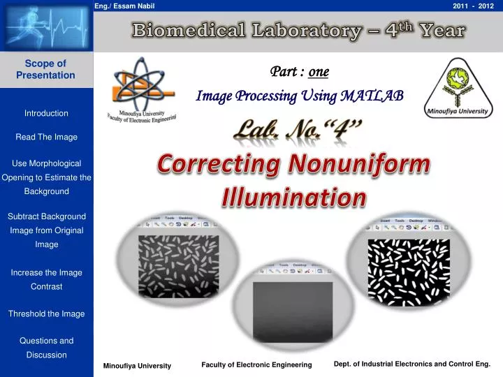
Biomedical Laboratory – 4th Year • Part : one • Image Processing Using MATLAB Lab. No.“4” Correcting Nonuniform Illumination
Introduction • Application: Using an image of rice grains, this example illustrates how you can enhance an image to correct for nonuniform illumination, then use the enhanced image to identify individual grains. Introduction • Procedural steps: Step 1: Read and Display the Image Step 2: Use Morphological Opening to Estimate the Background Step 3: Subtract Background Image from Original Image Step 4:Increase the Image Contrast Step 5:Threshold the Image
Step 1: Read and Display The Image 1.1 Key Commands: I = imread('filename.fmt') :reads a grayscale or color image specified by filename and format fmt and stores it into array variable I. If the file is not in the current folder, or in a folder on the MATLAB path, specify the full pathname as: I = imread(‘D:\pictures\asd.jpg’) Read The Image figure :creates a new figure object using default property values, and automatically becomes the current figure until a new figure is either created or called. imshow(I) :displays the stored image of the variable array I. title('string') :adds the title specified by ‘string’ at the top and in the center of the current axes or figure.
Step 1: Read and Display The Image 1.2 Step application: Read in the ‘rice.png' image and bring its data to workspace. • I = imread('rice.png'); figure, imshow(I) Read The Image
Step 2: Estimate the Background 2.1 Preface: Notice that the background illumination is brighter in the center of the image than at the bottom. Use imopen to estimate the background illumination. Use Morphological Opening to Estimate the Background 2.2 Key Commands: IM2 = imopen(IM,SE) performs morphological opening on the grayscale or binary image IM with the structuring element SE. 2.3 Step application: background =imopen(I,strel('disk',15));
Step 2: Estimate the Background Use Morphological Opening to Estimate the Background
Step 3: Subtract Background from Original 3.1 Preface: Notice that the background illumination is brighter in the center of the image than at the bottom. Use imopen to estimate the background illumination. 3.2 Step application: I2 = I – background; figure, imshow(I2); Subtract Background Image from Original Image OR I2 = imsubtract(I,background); figure, imshow(I2);
Step 4: Increase the Image Contrast 4.1 Step application: • I3 = imadjust(I2); • figure, imshow(I3); Increase the Image Contrast
Step 5: Threshold the Image 5.1 Preface: Create a new binary image by thresholding the adjusted image. 5.2 Step application: level = graythresh(I3); bw = im2bw(I3,level); figure, imshow(bw); • Threshold the Image
Questions and Discussion Questions and Discussion