Download
1 / 26
260 likes | 354 Views
Explore physics-based constraints in forward modeling analysis of time-correlated image data for accurate reconstructions. Experiment with radiographic imaging problems to compare to independent analysis approaches.

E N D
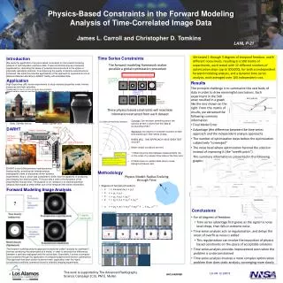
Physics-Based Constraints in the Forward Modeling Analysis of Time-Correlated Image Data (AMS 2012)James L. Carroll Chris D. Tomkins LA-UR 12-01365
Abstract • The forward-model approach has been shown to produce accurate reconstructions of scientific measurements for single-time image data. Here we extend the approach to a series of images that are correlated in time using the physics-based constraints that are often available with scientific imaging. The constraints are implemented through a representational bias in the model and, owing to the smooth nature of the physics evolution in the specified model, provide an effective temporal regularization. Unlike more general temporal regularization techniques, this restricts the space of solutions to those that are physically realizable. We explore the performance of this approach on a simple radiographic imaging problem of a simulated object evolving in time. We demonstrate that the constrained simultaneous analysis of the image sequence outperforms the independent forward modeling analysis over a range of degrees of freedom in the physics constraints, including when the physics model is under-constrained. Further, this approach outperforms the independent analysis over a large range of signal-to-noise levels.
Firing Point DARHT: Phase 2: “Second Axis” Optics and Detector Bunker Lab Space and Control Rooms Phase 1: “First Axis”
DARHT Axis 2 Accelerator • 2-ms, 2-kA, 18.4-MeV electron beam • for 4-pulse radiography. • Linear Induction Accelerator with wound Metglass cores and Pulse Forming Networks (PFNs) . • The Injector uses a MARX bank with 88 type E PFN stages at 3.2 MV. • Thermionic cathode. • 4 micropulses - variable pulse width. • Operations began in 2008.
Time Series Analysis • To date we have analyzed each element of DARHT axis 2 time series data independently • But we should be able to use information in the time series to compensate for some of the noise, and get better results.
A forward modeling approach is currently used in analysis of (single-time) radiographic data True radiographic physics ? How do we extract density from this transmission? Inverse approach (approximate physics) True density (unknown) Compare statistically Transmission (experimental) Simulated radiographic physics We develop a parameterized model of the density (parameters here might be edge locations, density values) Model density (allowed to vary) Transmission (simulated) Model parameters are varied so that the simulated radiograph matches the experiment
The forward-modeling framework makes possible a global optimization procedure Now, physics-based constraints on the evolution of the time-series data will also constrain the (global) solution Prior knowledge provides additional constraints at each time t1 t2 t3 t4 SOLUTION:Evaluated Density DATA: Transmission (experiment) Data constrain solution at each time t1 t2 t3 t4
t5 t4 t3 t2 t1 time These physics-based constraints will maximize information extracted from each dataset Concept: Can we learn something about the solution at time 3 (blue) from the data at surrounding times? Approach: use physics to constrain solution at each time based upon time-series of data. WHEN WILL THIS APPROACH HAVE GREATEST VALUE? When certain conditions are met: 1) Must have the time between measurements (Dt) on the order of a relevant time scale of the flow; and 2) Must have non-perfect data (due to noise, background levels, etc). Consider an evolving interface: Data must be correlated in time! Perfect data would be the only required constraint… (Noisier data means the global optimization adds more value).
Example • Graded Polygon:
Physics Model: Radius Evolving through Time • Degrees of Temporal Freedom: • 1: • 2: • 3: • 4: • … • n:
Simulated Expanding Object Simulated Data Radiograph Time Step 1 Simulated Data Radiograph Time Step 2 Simulated Data Radiograph Time Step 3 Simulated Data Radiograph Time Step 4 Densities Time Step 1 Densities Time Step 2 Densities Time Step 3 Densities Time Step 4 Unobserved Starting Position
Goal • Explore Relationships Between: • Degrees of temporal freedom • Noise • Optimization Difficulty
Challenge • To summarize the above and look for patterns and trends
Data Summary Approach: Final Error
Errors vs optimization steps for Various Noise levels for 2 DF
Time Series Results • 1DF: Simple TSA is always superior to static analysis • 2DF: Simple TSA is almost always superior to static analysis. • 3DF: Simple TSA is better with VERY high Signal to Noise Ratios, 1:10 at the edges, and 15:10 in the center. • Average SNR? • ≈7:10 • 4DF: Unknown… • Approaching an under/constrained problem
Time Series Results • Time series analysis involves a far more difficult optimization problem than is present in static analysis. • Interestingly enough, with lower noise levels the optimization problem is more “difficult” in the sense that it is possible to refine the answer to a greater degree • When the optimization problem can be solved, time series analysis can outperform static analysis for some combinations of noise and temporal degrees of freedom. • The number of optimization steps necessary before time series analysis outperforms static analysis depends on the noise and the temporal degrees of freedom.
Conclusions • Time series analysis shows potential for real applications at DARHT • Improvement will depend on the noise level present in the data. • Improvement will depend on how tightly the physics can constrain the temporal motion of the object • Complex global optimization will likely require improvements in the BIE’s function optimization algorithms
Future Work • Try imperfect physics. • Penalty term for deviation form time series prediction. • Explore higher temporal degrees of freedom • Analysis of more complex shapes • Implementation of more advanced function optimization routines • Exploration of other techniques for taking advantage of time series data besides fitting a polynomial.