CS151B Computer System Architecture
CS151B Computer System Architecture. Instructor: Savio Chau, Ph.D. Office: BH4531N Class Location: Class: Mon & Wed 4:00 - 6:00 p.m. Office Hour: Mon & Wed 6:00 - 7:00 p.m. TA1:. Syllabus. Reading Assignments. Note: Two sets of advanced topic slide are provided for reference.

CS151B Computer System Architecture
E N D
Presentation Transcript
CS151BComputer System Architecture Instructor: Savio Chau, Ph.D. Office: BH4531N Class Location: Class: Mon & Wed 4:00 - 6:00 p.m. Office Hour: Mon & Wed 6:00 - 7:00 p.m. TA1:
Reading Assignments Note: Two sets of advanced topic slide are provided for reference
Administrative Information • Text: • Patterson and Hennessy “Computer Organization and Design: The Hardware/Software Interface,” 2 ed. Morgan Kaufman, 1998 • Lecture Slides • Web Site: http://www.cs.ucla.edu/classes/spring03/csM151B/l1 • Grades • Homework 10% • Midterm 30% • Project 20% • Final 40% General grading guideline: A 80%, 80% > B 70%, 70% > C 60%, 60% > D 50%, 50% < F May change as we go along • References • Hennessy and Patterson, “Computer Architecture A Quantitative Approach,” 2nd Ed. Morgan Kaufman 1996 • Tanenbaum, “Structured Computer Organization,” 3d Ed., Prentice Hall 1990
Administrative Information Contact Information • Instructor: Savio Chau Email: savio.chau@jpl.nasa.gov • TA: Donald Lam Office: BH4428 Tel: 310 479 6553 Email: donaldl@cs.ucla.edu Homework: • Turn in the original of your homework to the following drop boxes on or before due day: • Discussion Class 2A: BH 4428, Box C-10 • Make a copy of your homework and turn it in to me on due day. The copy will be kept by me for record. (Too many students complained about TA losing their homework in the past.)
Homework Grading Policy • Unless consented by the instructor, homework that is up to 2 calendar days late will receive half credit. Homework more than 2 days late will receive no credit. • Homework must be reasonably tidy. Unreadable homework will not be graded • Unaided work on homework problems will be graded mainly based on effort. However, you must answer every part of the question, and the answer must address that part of the question. Always show your work, and make your answer as clear as possible. • Group work is OK. However: • Each member of the group MUST turn in his/her homework separately. • If you worked with other students on a question, you must state the names of all students in the group. Homework that have identical answers without this information may be investigated for violating the academic integrity policy, so please record any cooperation. • Group work on a homework problem will be graded on accuracy, and there will be deductions for mistakes. Each student should first attempt to answer every question on his or her own prior to meeting with the group or asking another student for help. After meeting with the group or seeking help, each student should verify the correctness of the answer
? Keyboard Controller What You Will Learn In This Course A Typical Computing Scenario You will Learn: • How to design processor to run programs Processor Processor Processor Execution Execution • The memory hierarchy to supply instructions and data to the processor as quickly as possible cache ? loaded Memory Array Computer Bus • The input and output of a computer system Hard Drive Hard Drive HD Controller HD Controller HD Controller • In-depth understanding of trade-offs at hardware-software boundary • Experience with the design process of a complex (hardware) design Power Supply Display Controller Display Controller Keyboard Controller Printer Controller Network Controller
What You Will Learn in This Lecture • What is Computer Architecture • Forces on Evolution of Computer Architecture • Measurement and Evaluation of Computer Performance • Number Representation • Brief Review of Logic Design
Control Application ALU Mem I Reg Operating System Software Compiler Firmware Instruction Set Architecture Vdd Instr. Set Proc. I/O system I1 O1 Datapath & Control Vdd I1 O1 Digital Design I2 O2 Hardware I1 O1 Circuit Design Physical Design What is Computer Architecture? • Coordination of many levels of abstraction • Under a rapidly changing set of forces • Design, Measurement, and Evaluation Bottom Up view Courtesy D. Patterson
Layer of Representations Program: temp = v[k]; v[k] = v[k+1]; v[k+1] = temp; High Level Language Program Top down view Compiler Assembly Program: Assembly Language Program lw $15, 0($2) lw $16, 4($2) sw $16, 0($2) sw $15, 4($2) Assembler Machine Language Program in Memory Object machine code Machine Language Program: Linker Executable machine code 0000 1001 1100 0110 1010 1111 0101 1000 1010 1111 0101 1000 0000 1001 1100 0110 1100 0110 1010 1111 0101 1000 0000 1001 0101 1000 0000 1001 1100 0110 1010 1111 Loader Instruction Set Architecture Machine Interpretation Control Signal Specification ALUOP[0:3] InstReg[9:11] & MASK Courtesy D. Patterson
Computer Architecture (Our Perspective) Computer Architecture = Instruction Set Architecture + Machine Organization • Instruction Set Architecture: the attributes of a [computing] system as seen by the programmer, i.e. the conceptual structure and functional behavior • Instruction Set • Instruction Formats • Data Types & Data Structures: Encodings & Representations • Modes of Addressing and Accessing Data Items and Instructions • Organization of Programmable Storage • Exceptional Conditions • Machine Organization:organization of the data flows and controls, the logic design, and the physical implementation. • Capabilities & Performance Characteristics of Principal Functional Unit (e.g., ALU) • Ways in which these components are interconnected • Information flows between components • Logic and means by which such information flow is controlled. • Choreography of Functional Units to realize the ISA • Register Transfer Level (RTL) Description
Forces on Computer Architecture Technology Programming Languages Computer Architecture Applications Operating Systems History Courtesy D. Patterson
100000000 10000000 R10000 Pentium R4400 i80486 1000000 i80386 Transistors i80286 100000 R3010 i80x86 i8086 SU MIPS M68K 10000 MIPS i4004 Alpha 1000 1965 1970 1975 1980 1985 1990 1995 2000 2005 Processor Technology logic capacity: about 30% per year clock rate: about 20% per year 1000 R10000 R4400 100 Pentium i80486 Clock (MHz) R3010 10 i80x86 1 M68K MIPS Alpha 0.1 1965 1970 1975 1980 1985 1990 1995 2000 Courtesy D. Patterson
Memory Technology DRAM capacity: about 60% per year (2x every 18 months) DRAM speed: about 10% per year DRAM Cost/bit: about 25% per year Disk capacity: about 60% per year Courtesy D. Patterson
How Technology Impacts Computer Architecture • Higher level of integration enables more complex architectures. Examples: • On-chip memory • Super scaler processors • Higher level of integration enables more application specific architectures (e.g., a variety of microcontrollers and DSPs) • Larger logic capacity and higher performance allow more freedom in architecture trade-offs. Computer architects can focus more on what should be done rather than worrying about physical constraints • Lower cost generates a wider market. Profitability and competition stimulates architecture innovations
Measurement and Evaluation Architecture is an iterative process -- searching the space of possible designs -- at all levels of computer systems Design Analysis Creativity Cost / Performance Analysis Good Ideas Mediocre Ideas Bad Ideas Courtesy D. Patterson
Seconds Instructions Cycles Seconds CPU time (execution time) = = Instructions Cycles Program Program Performance Analysis Basic Performance Equation: *Note: Different instructions may take different number of clock cycles. Cycle Per Instruction (CPI) is only an average and can be affected by application. Courtesy D. Patterson
Other ways to express CPU time: CPU Clock Cycles per Program CPU time = Clock Rate Instructions / Program CPI = Clock Rate = CPU Clock Cycles per Program / Clock Rate = CPU Clock Cycles per Program Cycle Time Other Useful Performance Metrics CPI = CPU Clock Cycles per Program / Instructions per Program = Average Number of Clock Cycles per Instruction CPU Clock Cycles per Program = Instrs per Program Average Clocks Per Instr. = Instructions / Program CPI = Ci CPIi for multiple programs See Class Example #1
Ex Time reference machine Relative MIPS = MIPS reference machine Ex Time target machine Traditional Performance Metrics • Million Instructions Per Second (MIPS) MIPS = Instruction Count / (Time 106) • Relative MIPS • Million Floating Point Operation Per Second (MFLOPS) MFLOPS = Floating Point Operations / (Time 106) • Million Operation Per Second (MOPS) MFLOPS = Operations / (Time 106)
(5+1+1) 109 (51+12+13) 109 20 sec; = 350 = 20 106 500 106 (10+1+1) 109 (101+12+13) 109 30 sec; = 400 = 30 106 500 106 MIPS • Advantage: Intuitively simple (until you look under the cover) • Disadvantages: • Doesn’t account for differences in instruction capabilities • Doesn’t account for differences in instruction mix • Can vary inversely with performance Example: Two processors, both are 500 MHz, are running the same program. But the program is compiled into different number of machine instructions on the two processors due to their different instruction set architecture. MIPS1 = CPU Time1 = MIPS2 = CPU Time2 =
Benchmarks • Compare performance of two computers by running the same set of representative programs • Good benchmark provides good targets for development. Bad benchmark cannot identify speedup that helps real applications • Benchmark Programs • (Toy) Benchmarks • 10 to 100 Line Programs • e. g., Sieve, Puzzle, Quicksort • Synthetic Benchmarks • Attempt to Match Average Frequencies of Real Workloads • e. g., Whetstone, dhrystone • Kernels • Time Critical Excerpts of Real Programs • e. g., Livermore Loops • Real Programs • e. g., gcc, spice
Successful Benchmark: SPEC • 1987 RISC Industry Mired in “benchmarking”: (“ That is an 8-MIPS Machine, but they claim 10-MIPS!”) • EE Times + 5 Companies Band Together to Form Systems Performance Evaluation Committee (SPEC) in 1988: Sun, MIPS, HP, Apollo, DEC • Create Standard List of Programs, Inputs, Reporting: • Some Real programs • Includes OS Calls • Some I /O
Exec. Time on Test System Spec Ratio for Each Program = Exec Time on Vax–11/ 780 Specmark = Geometric Mean of all 10 SPEC ratios = n P 10 SPEC Ratio (i) i = 1 1989 SPEC Benchmark • 10 Programs • 4 Logical and Fixed Point Intensive Programs • 6 Floating Point Intensive Programs • Representation of Typical Technical Applications • Evolution since 1989 • 1992: SpecInt92 (6 Integer Programs), SpecFP92 (14 Floating Point Programs) • 1995: New Program Set, “Benchmarks Useful for 3 Years”
Why Geometric Mean? • Reason for SPEC to use geometric mean: • SPEC has to combine the normalized execution time of 10 programs. Geometric means is able to summarize normalized performance of multiple programs more consistently • Disadvantage: Not intuitive, cannot easily relate to actual execution time Example: Compare speedup on Machine A and Machine B B is 10 times faster than A running Program 1, but A is 10 times faster than B running Program 2. Therefore, two computers should have same speedup. This is indicated by the geometric mean but not by the arithmetic mean (in fact, the arithmetic mean will be affected by the choice of reference machine)
F F (1 - F) + (1 - F) + S S Amdhal’s Law Speedup Due to Enhancement E: Ex time (without E) Performance (with E) Speedup(E) = = Ex time (with E) Performance (without E) Suppose that Enhancement E accelerates a Fraction F of the task by a factor S and the remainder of the Task is unaffected then: Ex time (without E) Ex time (with E) = Ex time (without E) Ex time (without E) = Speedup (with E) = Ex time (with E) Ex time (without E) Courtesy D. Patterson
Amdhal’s Law Example • A real case (modified): • A project uses a computer which as a processor with performance of 20 ns/instruction (average) and a memory with 20 ns/access (average). A new project decides to use a new computer which has a processor with an advertised performance 10 times faster than the old processor. However, no improvement was made in memory. What is the expected performance and the real performance of the new computer? • Answer: • Performance old computer = 1 instructon / (20 ns + 20 ns) = 25 MIPS • Since the new processor is 10 times faster, the expected performance of the new computer would have been 250 MIPS. However, since the memory speed has not been improved, • Real Speedup = (20 ns + 20 ns) / (2 ns + 20 ns) = 1.8 • Actual Performance new computer = 25 MIPS 1.8 = 45 MIPS • Less than 2 times of the old computer!
Number Representations • Unsigned: The N-bit word is interpreted as a non-negative integer Value = bn-12n-1 bn-22n-2 … b121 b020 b-12-1 … bm2-m Example: Represent value of 101100112 in decimal number Value = 127 026 125 124 023 022 121 120 = 17910 Example: Convert 2810 to binary Quotion Remainder 28 2 0 (LSB) 14 2 0 7 2 1 3 2 1 1 2 1 (MSB) 2810 = 111002 Example: Convert 0.812510 to binary Decimal One’s 0.8125 2 = 1.625 1 (MSB) 0.625 2 = 1.25 1 0.25 2 = 0.5 0 0.5 2 = 1 1 (LSB) 0.812510 = 0.11012
For fixed point number only, normalized floating point number is more complicate Number Representations • Negative Integers: Two’s complement Value = s2n bn-12n-1 bn-22n-2 … b121 b020; s = sign bit • Simple sign detection because there is only 1 representation of zero (as oppose to 1’s complement) • Negation: bitwise toggle and add 1 (i.e., 1’s complement + 1) • Visual shortcut for negation • Find least significant non-zero bit • Toggle all bits more significant than the least significant non-zero bit • Example 8-bit word: 88 = [0][1011000] 88 = [1][0101000] • Two’s complement Operations • Add: X+Y=Z, set Carry-In = 0, Overflow if signs of X and Y are the same but the sign of Z is different: (Xn-1= Yn-1) and (Xn-1!= Zn-1) • Right Shift [1]001002 [1]100102 [1]110012 • Left Shift [1]101002 [1]010102 [1]001012 • Sign Extension [1]001002 [1]11111111111001002 5 bits 16 bits
Number Representations • Floating Point Numbers Three parts: sign(s), mantissa (F), exponent (E) Value = (1)s F 2 E Example 1: Represent 36410 as a floating point number: If s =1 bit, F = 7 bits, E = 2 bits; range = 127 222-1 = 1016 36410 = 1 9110 2 2 = [1][1011011][10]2 If s =1 bit, F = 6 bits, E = 3 bits; range = 63 223-1 = 8064 36410 = 1 4510 2 3 = [1][101101][011]2 Example 2: s = 1, F = 10110112 = 9110, E = 011010012 = 10510 [1][1011011][01101001]2 = 9110 210510= 3.6910 1033 • Normalized Floating Point Numbers: F = 1.DDD···, where D = 1 or 0, decimal part = significand Example: s = 1, F =1.0110112 , E = 011010012 [1][1011011][01101001]2 = 1.42187510 210510= 1.7110 1031 Losing precision but gaining range
Floating Point Operations (Base 10) • Addition (Subtraction) • Step 1: Align decimal point of the number with smaller exponent A = 9.99910 10 1, B = 1.61010 10 1 0.01610 10 1 • Step 2: Add (subtract) mantissas C =A + B = (9.99910+ 0.01610) 10 1 = 10.01510 10 1 • Step 3: Renormalize the sum (difference) C = 10.01510 10 1 1.001510 10 2 • Step 4: Round the sum (difference) C = 1.001510 10 2 1.00210 10 2 • Multiplication (Division) • Step 1: Add (subtract) exponents A = 1.11010 10 10, B = 9.20010 10 5, New exponent = 10 + (- 5) = 5 • Step 2: Multiply (divide) mantissas 1.11010 9.20010 = 10.21210 • Step 3: Renormalize the product (quotion) 10.21210 10 5 1.021210 10 6 • Step 4: Round the product (quotion) 10.21210 10 6 1.02110 10 6 • Step 5: Determine the sign Both signs are + Sign of produce is +
Overflow in Normalized Floating Point Numbers • If two normalized floating point numbers have opposite signs, their sum will never overflow. Example Sign Mantissa Exponent -1.5 = (-1)1 x 1.101 x 22 1 1. 1 0 1 1 0 7 = (-1)0 x 1.110 x 22 + 0 1. 1 1 0 1 0 Check: 7 – 1.5 = 5.5 = (-1)0 x 1.011 x 22 1 0 1. 0 1 1 1 0 Drop this bit because overflow cannot happen carry • If two normalized floating point numbers have the same sign, their sum may overflow (sign A = sign B sign of sum). But in floating point, the overflow can be removed by re-normalization, unless the exponent is already maximum. Example: Sign Mantissa Exponent 6.5 = (-1)0 x 1.101 x 22 0 1. 1 0 1 1 0 7 = (-1)0 x 1.110 x 22 + 0 1. 1 1 0 1 0 Check: 7 + 6.5 = 13.5 = (-1)0 x 1.1011 x 22 0 1. 0 1 1 1 0 0 1. 1 0 1 1 1 Re-normalize If this bit is carried to the sign bit, it will cause overflow. But the overflow can be removed by normalization 1 carry
IEEE 754 Standard for Floating Point Numbers Single precision format: • Maximize precision of representation with fix number of bits • Gain 1 bit by making leading 1 of mantissa implicit. Therefore, F = 1 + significand, Value = (1)s (1 + significand) 2 E • Easy for comparing numbers • Put sign bit at MSB • Use bias instead of sign bit for exponent field Real exponent value = exponent – bias. Bias = 127 for single precision Examples: IEEE 754 Floating Point Number Value Exponent A = -12600000001 (1)s F 2 (1-127) = (1)s F 2-126 Exponent B = 127 11111110 (1)s F 2 (254-127) = (1)s F 2127 This is much easier to compare than having A = 12610 = 100000102 and B = 12710 = 011111112 sign Exponent (biased) Significand only (leading 1 is implicit) Other formats: Double (64 bits), Double Extended (>80 bits), Quadruple (128 bits) See Class Example
IEEE 754 Computation Example A) 40 = (–1)0 1. 25 25 = (–1)0 1.012 2(132 – 127) = [0][10000100][101000000000000000000] B) –80 = (–1)1 1. 25 26 = (–1)1 1. 012 2(133 – 127) = [1][10000101][111101000000000000000] C) Remove normalization of one of the significands so that the exponents can be aligned: 40 = (–1)0 0. 3125 27 = (–1)0 0.01012 2 (134 – 127) = [0][10000110][010100000000000000000] –80 = (–1)1 0. 6250 27 = (–1)1 0.10102 2 (134 – 127) = [1][10000110][101000000000000000000] D) Need to convert the IEEE 754 significand of –80 into 2’s complement before the subtraction: –80 = [1][10000110][101000000000000000000] [1][10000110][011000000000000000000] 40 – 80 = [0][10000110][010100000000000000000] + [1][10000110][011000000000000000000] = [0][10000110][101100000000000000000] E) Convert the result in 2’s complement into IEEE 754 = [1][10000110][010100000000000000000] F) Renormalize: [1][10000110][010100000000000000000] = [1][10000100][010000000000000000000] = (–1)1 1.012 25 Check: 40 – 80 = – 40 = (–1)1 1.25 25 = (–1)1 1.012 25
Special Numbers in IEEE 754 Standard Number Type Sign Bit Exponent Nth bit (Hidden) Significand NaNs (Not a Number) X 111...111 1 1xxx...xxx SNaNs (Signaling Not a Number) X 111...111 1 Non-zero 0xxx...xxx Infinities ± 111...111 1 0 Subnormals (Very small numbers) ± 0 0 (denormalized) positive n < 2N-1 N=size of significand+1 Zeros ± 0 0 0 Note: NaNs is used to indicate invalid data and SNaNs is used to indicate invalid operations
cin sum a b cout op code sum cin 0 a b a 1 b a + b 2 output cout a · b 3 next cell 1-Bit ALU Design • A 1-bit adder sum = a b carry-in, carry-out = (a · b) + (a · carry-in) + (b · carry-in) • A 1-bit ALU with AND, OR, XOR
Multiple-Bit ALU Design • Ripple Carry ALU: Too slow. Not used in real machines A3 B3 A2 B2 A1 B1 A0 B0 C0 1-bit ALU 1-bit ALU 1-bit ALU 1-bit ALU Op Code C4 C3 C2 C1 Out3 Out2 Out1 Out0 • Carry Look Ahead ALU A3 B3 A2 B2 A1 B1 A0 B0 C0 1-bit ALU 1-bit ALU 1-bit ALU 1-bit ALU Op Code C4 Carry Look Ahead Logic P3 G3 C3 P2 G2 C2 P1 G1 C1 P0 G0 Out3 Out2 Out1 Out0
![Computer Architecture &amp; Operating System [O.S.]](https://cdn0.slideserve.com/35278/computer-architecture-operating-system-o-s-dt.jpg)