Chapter 4 Network Layer
Chapter 4 Network Layer. Computer Networking: A Top Down Approach 4 th edition. Jim Kurose, Keith Ross Addison-Wesley, July 2007. . Computer Networking: A Top Down Approach 5 th edition. Jim Kurose, Keith Ross Addison-Wesley, April 2009. . transport segment from sending to receiving host

Chapter 4 Network Layer
E N D
Presentation Transcript
Chapter 4Network Layer Computer Networking: A Top Down Approach 4th edition. Jim Kurose, Keith RossAddison-Wesley, July 2007. Computer Networking: A Top Down Approach 5th edition. Jim Kurose, Keith RossAddison-Wesley, April 2009. Network Layer
transport segment from sending to receiving host on sending side encapsulates segments into datagrams on rcving side, delivers segments to transport layer network layer protocols in every host, router router examines header fields in all IP datagrams passing through it network data link physical network data link physical network data link physical network data link physical network data link physical network data link physical network data link physical network data link physical network data link physical network data link physical network data link physical application transport network data link physical application transport network data link physical Network layer Network Layer
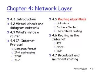
Two Key Network-Layer Functions • 1. forwarding: move packets from router’s input to appropriate router output • 2. routing: determine route taken by packets from source to dest. • routing algorithms • before packets arrive • 3. connection setup: for some connection-oriented architectures (ATM, x.25) • Before datagrams flow • Establishes a virtual circuit (VC) Network Layer
Example services for individual datagrams: guaranteed delivery guaranteed delivery with less than 40 msec delay Example services for a flow of datagrams: in-order datagram delivery guaranteed minimum bandwidth to flow restrictions on changes in inter-packet spacing Network service model Q: What service model for “channel” transporting datagrams from sender to receiver? Network Layer
Network layer service models: Guarantees ? Network Architecture Internet ATM ATM ATM ATM Service Model best effort CBR VBR ABR UBR Congestion feedback no (inferred via loss) no congestion no congestion yes no Bandwidth none constant rate guaranteed rate guaranteed minimum none Loss no yes yes no no Order no yes yes yes yes Timing no yes yes no no Network Layer
call setup, teardown for each call before data can flow each packet carries VC identifier (not destination host address) every router on source-dest path maintains “state” for each passing connection link, router resources (bandwidth, buffers) may be allocated to VC (dedicated resources = predictable service) Yet still uses statistical multiplexing “source-to-dest path behaves much like telephone circuit” performance-wise network actions along source-to-dest path Virtual circuits Network Layer
VC number 22 32 12 3 1 2 interface number Incoming interface Incoming VC # Outgoing interface Outgoing VC # 1 12 3 22 2 63 1 18 3 7 2 17 1 97 3 87 … … … … Forwarding table Forwarding table in northwest router: Routers maintain connection state information! Network Layer
used to setup, maintain teardown VC used in ATM, frame-relay, X.25 not used in today’s Internet application transport network data link physical application transport network data link physical Virtual circuits: signaling protocols 6. Receive data 5. Data flow begins 4. Call connected 3. Accept call 1. Initiate call 2. incoming call Network Layer
no call setup at network layer routers: no state about end-to-end connections no network-level concept of “connection” packets forwarded using destination host address packets between same source-dest pair may take different paths application transport network data link physical application transport network data link physical Datagram networks 1. Send data 2. Receive data Network Layer
Internet (datagram) data exchange among computers “elastic” service, no strict timing req. “smart” end systems (computers) can adapt, perform control, error recovery simple inside network, complexity at “edge” many link types different characteristics uniform service difficult ATM (VC) evolved from telephony human conversation: strict timing, reliability requirements need for guaranteed service “dumb” end systems telephones complexity inside network Datagram or VC network: why? Network Layer
Router Architecture Overview Two key router functions: • run routing algorithms/protocol (RIP, OSPF, BGP) • forwarding datagrams from incoming to outgoing link Network Layer
Three types of switching fabrics 1st generation, memory bottleneck, limited speed Bus bottleneck, 32Gbps Interconnection network, 60Gbps Network Layer
Input Port Queuing • Fabric slower than input ports combined -> queueing may occur at input queues • Head-of-the-Line (HOL) blocking: queued datagram at front of queue prevents others in queue from moving forward • queueing delay and loss due to input buffer overflow! Network Layer
Host, router network layer functions: • ICMP protocol • error reporting • router “signaling” • IP protocol • addressing conventions • datagram format • packet handling conventions • Routing protocols • path selection • RIP, OSPF, BGP forwarding table The Internet Network layer Transport layer: TCP, UDP Network layer Link layer physical layer Network Layer
IP protocol version number 32 bits total datagram length (bytes) header length (bytes) type of service head. len ver length for fragmentation/ reassembly fragment offset “type” of data flgs 16-bit identifier max number remaining hops (decremented at each router) upper layer time to live header checksum 32 bit source IP address 32 bit destination IP address upper layer protocol to deliver payload to E.g. timestamp, record route taken, specify list of routers to visit. Options (if any) data (variable length, typically a TCP or UDP segment) IP datagram format how much overhead with TCP? • 20 bytes of TCP • 20 bytes of IP • = 40 bytes + app layer overhead Network Layer
network links have MTU (max.transfer size) - largest possible link-level frame. different link types, different MTUs large IP datagram divided (“fragmented”) within net one datagram becomes several datagrams “reassembled” only at final destination IP header bits used to identify, order related fragments IP Fragmentation & Reassembly fragmentation: in: one large datagram out: 3 smaller datagrams reassembly Network Layer
length =1500 length =1040 length =1500 length =4000 ID =x ID =x ID =x ID =x fragflag =0 fragflag =0 fragflag =1 fragflag =1 offset =0 offset =185 offset =0 offset =370 One large datagram becomes several smaller datagrams IP Fragmentation and Reassembly Example • 4000 byte datagram • MTU = 1500 bytes 1480 bytes in data field offset = 1480/8 Network Layer
IP address: 32-bit identifier for host, router interface interface: connection between host/router and physical link router’s typically have multiple interfaces host typically has one interface IP addresses associated with each interface 223.1.1.2 223.1.2.2 223.1.2.1 223.1.3.2 223.1.3.1 223.1.3.27 IP Addressing: introduction 223.1.1.1 223.1.2.9 223.1.1.4 223.1.1.3 223.1.1.1 = 11011111 00000001 00000001 00000001 223 1 1 1 Network Layer
IP address: subnet part (high order bits) host part (low order bits) What’s a subnet ? device interfaces with same subnet part of IP address can physically reach each other without intervening router Subnets 223.1.1.1 223.1.2.1 223.1.1.2 223.1.2.9 223.1.1.4 223.1.2.2 223.1.1.3 223.1.3.27 subnet 223.1.3.2 223.1.3.1 network consisting of 3 subnets Network Layer
host part subnet part 11001000 0001011100010000 00000000 200.23.16.0/23 IP addressing: CIDR CIDR:Classless InterDomain Routing • subnet portion of address of arbitrary length • address format: a.b.c.d/x, where x is # bits in subnet portion of address Network Layer
IP addresses: how to get one? Q: How does host get IP address? • hard-coded by system admin in a file • Wintel: control-panel->network->configuration->tcp/ip->properties • UNIX: /etc/rc.config • DHCP:Dynamic Host Configuration Protocol: dynamically get address from as server • “plug-and-play” Network Layer
200.23.16.0/23 200.23.18.0/23 200.23.30.0/23 200.23.20.0/23 . . . . . . Hierarchical addressing: route aggregation Hierarchical addressing allows efficient advertisement of routing information: Organization 0 Organization 1 “Send me anything with addresses beginning 200.23.16.0/20” Organization 2 Fly-By-Night-ISP Internet Organization 7 “Send me anything with addresses beginning 199.31.0.0/16” ISPs-R-Us Network Layer
2 4 1 3 S: 138.76.29.7, 5001 D: 128.119.40.186, 80 S: 10.0.0.1, 3345 D: 128.119.40.186, 80 1: host 10.0.0.1 sends datagram to 128.119.40.186, 80 2: NAT router changes datagram source addr from 10.0.0.1, 3345 to 138.76.29.7, 5001, updates table S: 128.119.40.186, 80 D: 10.0.0.1, 3345 S: 128.119.40.186, 80 D: 138.76.29.7, 5001 NAT: Network Address Translation NAT translation table WAN side addr LAN side addr 138.76.29.7, 5001 10.0.0.1, 3345 …… …… 10.0.0.1 10.0.0.4 10.0.0.2 138.76.29.7 10.0.0.3 4: NAT router changes datagram dest addr from 138.76.29.7, 5001 to 10.0.0.1, 3345 3: Reply arrives dest. address: 138.76.29.7, 5001 Network Layer
NAT: Network Address Translation • 16-bit port-number field: • 60,000 simultaneous connections with a single LAN-side address! • NAT is controversial: • routers should only process up to layer 3 • violates end-to-end argument • NAT possibility must be taken into account by app designers, eg, P2P applications • address shortage should instead be solved by IPv6 Network Layer
NAT traversal problem • client want to connect to server with address 10.0.0.1 • server address 10.0.0.1 local to LAN (client can’t use it as destination addr) • only one externally visible NATted address: 138.76.29.7 • Solutions: 1. statically configure NAT to forward incoming connection requests at given port to server • e.g., (138.76.29.7, port 2500) always forwarded to 10.0.0.1 port 25000 • 2. use UPnP to automate 1 • 3. use relay: used in p2p 10.0.0.1 Client ? 10.0.0.4 138.76.29.7 NAT router Network Layer
NAT traversal problem • solution 3: relaying (used in Skype) • NATed server establishes connection to relay • External client connects to relay • relay bridges packets between to connections 2. connection to relay initiated by client 1. connection to relay initiated by NATted host 10.0.0.1 3. relaying established Client 138.76.29.7 NAT router Network Layer
IPv6 • Initial motivation:32-bit address space soon to be completely allocated. • Additional motivation: • header format helps speed processing/forwarding • header changes to facilitate QoS IPv6 datagram format: • fixed-length 40 byte header • no fragmentation allowed Network Layer
IPv6 Header (Cont) Priority: identify priority among datagrams in flow Flow Label: identify datagrams in same “flow.” (concept of“flow” not well defined). Next header: identify upper layer protocol for data Network Layer
Transition From IPv4 To IPv6 • Not all routers can be upgraded simultaneously • How will the network operate with mixed IPv4 and IPv6 routers? • Tunneling: IPv6 carried as payload in IPv4 datagram among IPv4 routers Network Layer
Flow: X Src: A Dest: F data Flow: X Src: A Dest: F data Flow: X Src: A Dest: F data Flow: X Src: A Dest: F data A B E F F A B E C D Src:B Dest: E Src:B Dest: E Tunneling tunnel Logical view: IPv6 IPv6 IPv6 IPv6 Physical view: IPv6 IPv6 IPv6 IPv6 IPv4 IPv4 A-to-B: IPv6 E-to-F: IPv6 B-to-C: IPv6 inside IPv4 B-to-C: IPv6 inside IPv4 Network Layer
routing algorithm local forwarding table header value output link 0100 0101 0111 1001 3 2 2 1 value in arriving packet’s header 1 0111 2 3 Interplay between routing, forwarding Network Layer
5 3 5 2 2 1 3 1 2 1 x z w y u v Graph abstraction Graph: G = (N,E) N = set of routers = { u, v, w, x, y, z } E = set of links ={ (u,v), (u,x), (v,x), (v,w), (x,w), (x,y), (w,y), (w,z), (y,z) } Remark: Graph abstraction is useful in other network contexts Example: P2P, where N is set of peers and E is set of TCP connections Network Layer
5 3 5 2 2 1 3 1 2 1 x z w y u v Graph abstraction: costs • c(x,x’) = cost of link (x,x’) • - e.g., c(w,z) = 5 • cost could always be 1, or • inversely related to bandwidth, • or inversely related to • congestion Cost of path (x1, x2, x3,…, xp) = c(x1,x2) + c(x2,x3) + … + c(xp-1,xp) Question: What’s the least-cost path between u and z ? Routing algorithm: algorithm that finds least-cost path Network Layer
Global or decentralized information? Global: all routers have complete topology, link cost info “link state” algorithms Decentralized: router knows physically-connected neighbors, link costs to neighbors iterative process of computation, exchange of info with neighbors “distance vector” algorithms Static or dynamic? Static: routes change slowly over time Dynamic: routes change more quickly periodic update in response to link cost changes Routing Algorithm classification Network Layer
Dijkstra’s algorithm net topology, link costs known to all nodes accomplished via “link state broadcast” all nodes have same info computes least cost paths from one node (‘source”) to all other nodes gives forwarding table for that node iterative: after k iterations, know least cost path to k dest.’s Notation: c(x,y): link cost from node x to y; = ∞ if not direct neighbors D(v): current value of cost of path from source to dest. v p(v): predecessor node along path from source to v N': set of nodes whose least cost path is definitively known A Link-State Routing Algorithm Network Layer
Dijsktra’s Algorithm 1 Initialization: 2 N' = {u} 3 for all nodes v 4 if v adjacent to u 5 then D(v) = c(u,v) 6 else D(v) = ∞ 7 8 Loop 9 find w not in N' such that D(w) is a minimum 10 add w to N' 11 update D(v) for all v adjacent to w and not in N' : 12 D(v) = min( D(v), D(w) + c(w,v) ) 13 /* new cost to v is either old cost to v or known 14 shortest path cost to w plus cost from w to v */ 15 until all nodes in N' Network Layer
5 3 5 2 2 1 3 1 2 1 x z w u y v Dijkstra’s algorithm: example D(v),p(v) 2,u 2,u 2,u D(x),p(x) 1,u D(w),p(w) 5,u 4,x 3,y 3,y D(y),p(y) ∞ 2,x Step 0 1 2 3 4 5 N' u ux uxy uxyv uxyvw uxyvwz D(z),p(z) ∞ ∞ 4,y 4,y 4,y Network Layer
Distance Vector Algorithm Bellman-Ford Equation (dynamic programming) Define dx(y) := cost of least-cost path from x to y Then dx(y) = min {c(x,v) + dv(y) } where min is taken over all neighbors v of x v Network Layer
Distance vector algorithm (4) Basic idea: • Each node periodically sends its own distance vector estimate to neighbors • When a node x receives new DV estimate from neighbor, it updates its own DV using B-F equation: Dx(y) ← minv{c(x,v) + Dv(y)} for each node y ∊ N Network Layer
Iterative, asynchronous: each local iteration caused by: local link cost change DV update message from neighbor Distributed: each node notifies neighbors only when its DV changes neighbors then notify their neighbors if necessary wait for (change in local link cost or msg from neighbor) recompute estimates if DV to any dest has changed, notify neighbors Distance Vector Algorithm (5) Each node: Network Layer
cost to x y z x 0 2 7 y from ∞ ∞ ∞ z ∞ ∞ ∞ 2 1 7 z x y Dx(z) = min{c(x,y) + Dy(z), c(x,z) + Dz(z)} = min{2+1 , 7+0} = 3 Dx(y) = min{c(x,y) + Dy(y), c(x,z) + Dz(y)} = min{2+0 , 7+1} = 2 node x table cost to x y z x 0 2 3 y from 2 0 1 z 7 1 0 node y table cost to x y z x ∞ ∞ ∞ 2 0 1 y from z ∞ ∞ ∞ node z table cost to x y z x ∞ ∞ ∞ y from ∞ ∞ ∞ z 7 1 0 time Network Layer
cost to x y z x 0 2 7 y from ∞ ∞ ∞ z ∞ ∞ ∞ 2 1 7 z x y Dx(z) = min{c(x,y) + Dy(z), c(x,z) + Dz(z)} = min{2+1 , 7+0} = 3 Dx(y) = min{c(x,y) + Dy(y), c(x,z) + Dz(y)} = min{2+0 , 7+1} = 2 node x table cost to cost to x y z x y z x 0 2 3 x 0 2 3 y from 2 0 1 y from 2 0 1 z 7 1 0 z 3 1 0 node y table cost to cost to cost to x y z x y z x y z x ∞ ∞ x 0 2 7 ∞ 2 0 1 x 0 2 3 y y from 2 0 1 y from from 2 0 1 z z ∞ ∞ ∞ 7 1 0 z 3 1 0 node z table cost to cost to cost to x y z x y z x y z x 0 2 7 x 0 2 3 x ∞ ∞ ∞ y y 2 0 1 from from y 2 0 1 from ∞ ∞ ∞ z z z 3 1 0 3 1 0 7 1 0 time Network Layer
Message complexity LS: with n nodes, E links, O(nE) msgs sent DV: exchange between neighbors only convergence time varies Speed of Convergence LS: O(n2) algorithm requires O(nE) msgs may have oscillations DV: convergence time varies may be routing loops count-to-infinity problem Robustness: what happens if router malfunctions? LS: node can advertise incorrect link cost each node computes only its own table DV: DV node can advertise incorrect path cost each node’s table used by others error propagate thru network Comparison of LS and DV algorithms Network Layer
scale: with 200 million destinations: can’t store all dest’s in routing tables! routing table exchange would swamp links! administrative autonomy internet = network of networks each network admin may want to control routing in its own network Hierarchical Routing Our routing study thus far - idealization • all routers identical • network “flat” … not true in practice Network Layer
aggregate routers into regions, “autonomous systems” (AS) routers in same AS run same routing protocol “intra-AS” routing protocol routers in different AS can run different intra-AS routing protocol Gateway router Direct link to router in another AS Hierarchical Routing Network Layer
forwarding table configured by both intra- and inter-AS routing algorithm intra-AS sets entries for internal dests inter-AS & Intra-As sets entries for external dests 3a 3b 2a AS3 AS2 1a 2c AS1 2b 3c 1b 1d 1c Inter-AS Routing algorithm Intra-AS Routing algorithm Forwarding table Interconnected ASes Network Layer
2c 2b 3c 1b 1d 1c Example: Setting forwarding table in router 1d • suppose AS1 learns (via inter-AS protocol) that subnet x reachable via AS3 (gateway 1c) but not via AS2. • inter-AS protocol propagates reachability info to all internal routers. • router 1d determines from intra-AS routing info that its interface I is on the least cost path to 1c. • installs forwarding table entry (x,I) … x 3a 3b 2a AS3 AS2 1a AS1 I Network Layer
Intra-AS Routing • also known as Interior Gateway Protocols (IGP) • most common Intra-AS routing protocols: • RIP: Routing Information Protocol • OSPF: Open Shortest Path First • IGRP: Interior Gateway Routing Protocol (Cisco proprietary) Network Layer
u v destinationhops u 1 v 2 w 2 x 3 y 3 z 2 w x z y C A D B RIP ( Routing Information Protocol) • distance vector algorithm • included in BSD-UNIX Distribution in 1982 • distance metric: # of hops (max = 15 hops) From router A to subsets: Network Layer
RIP advertisements • distance vectors: exchanged among neighbors every 30 sec via Response Message (also called advertisement) • ech advertisement: list of up to 25 destination nets within AS If no advertisement heard after 180 sec --> neighbor/link declared dead • routes via neighbor invalidated • new advertisements sent to neighbors • neighbors in turn send out new advertisements (if tables changed) Network Layer