Download
1 / 47
1.05k likes | 1.84k Views
Structural Equation Model[l]ing (SEM).

E N D
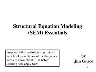
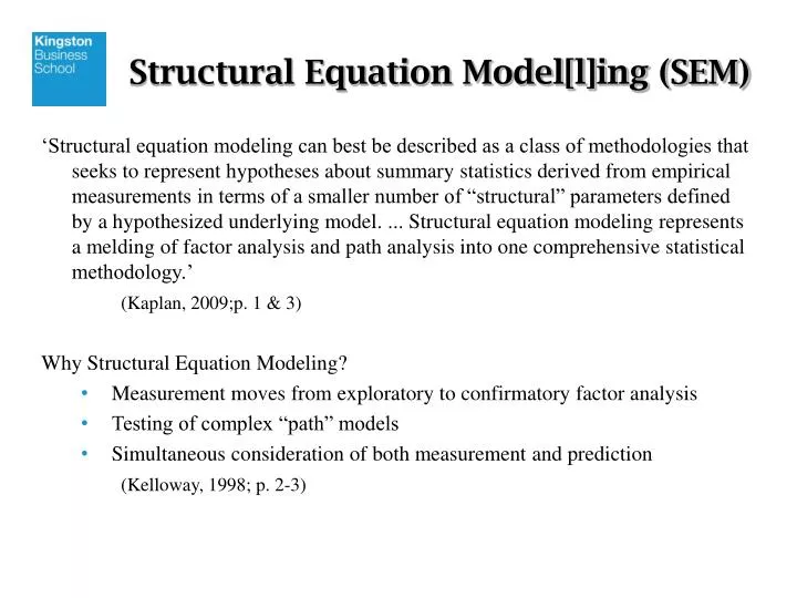
Structural Equation Model[l]ing (SEM) ‘Structural equation modeling can best be described as a class of methodologies that seeks to represent hypotheses about summary statistics derived from empirical measurements in terms of a smaller number of “structural” parameters defined by a hypothesized underlying model. ... Structural equation modeling represents a melding of factor analysis and path analysis into one comprehensive statistical methodology.’ (Kaplan, 2009;p. 1 & 3) Why Structural Equation Modeling? • Measurement moves from exploratory to confirmatory factor analysis • Testing of complex “path” models • Simultaneous consideration of both measurement and prediction (Kelloway, 1998; p. 2-3)
Approach to SEM (Kaplan, 2009; p. 9) Theory Model Specification Sample and Measures Estimation Assessment of fit Modification Discussion
A Typical SEM ‘Problem’ Appearance Taste Food Quality Regression weights Portion Size Satisfaction Correlation Loadings Friendly Employees Service Quality Competent Employees Courteous Employees = latent or unobservable or construct or concept or factor = directly observable variable
Latent and Observable Variables RLV FLV 1 2 3 4 1 2 3 4 X1 X2 X3 X4 X1 X2 X3 X4 The indicators are viewed as causing rather than being caused by the underlying LV … a change in the LV is not necessarily accompanied by a change in all its indicators, rather if any one of the indicators changes, then the latent variable would also change. FLVs represent emergent constructs that are formed from a set of indicators that may or may not have theoretical rationale. Inter-dependence amongst the indicators is not desired. Low correlation is expected amongst the indicators. The’s are regression weights The indicators are considered to be influenced, affected or caused by the underlying LV … a change in the LV will be reflected in a change in all indicators …there is a correspondence between the LV and its indicators (i.e., the indicators are seen as empirical surrogates for a LV). The underlying assumption is that the LV theoretically exists, rather than being constructed, and it is manifested through its indicators. High correlation is expected amongst the indicators. The ’s are correlations
Exogenous (independent) and Endogenous (dependent) Variables error2 error1 Measurement or Outer model: Relationship between the observed variables and their LVs 1 x1 x2 x3 1 1 1 2 y1 y2 y3 y4 y5 y6 2 Structural or Inner model: “Theoretically” grounded relationships between LVs x4 x5 x6
Mediation and Moderation error 1 error 2 1 1 Education Income Satisfaction error 1 Mediation 1 error 2 Income Partial Moderation 1 Education Satisfaction Full Moderation error 1 Income 1 Education Satisfaction
Covariance (CB-SEM) and Partial Least Squares (PLS-SEM) “ML [CBSEM] is theory-oriented and emphasises the transition from exploratory to confirmatory analysis. PLS is primarily intended for causal-predictive analysis in situations of high complexity but low theoretical information” (Joreskog & Wold, 1982; 270) “Such covariance-based SEM (CBSEM) focuses on estimating a set of model parameters so that the theoretiacl covariance matrix implied by the system of structural equations is as close as possible to the empirical covariance matrix observed within the estimation sample. ... Unline CBSEM PLS analysis does not work with latent variables, and estimates model parameters to maximize the variance explained for all endogenous constructs in the model through a series of ordinary least squares (OLS) regressions.” (Reinartz, Haenlein & Jenseler, 2009; 332)
HBAT DATA CUSTOMER SURVEY - HBAT is a manufacturer of paper products. Data from 100 randomly selected customers were collected on the following variables. Classification Variables/Emporographics X1 - Customer Type: Length of time a particular customer has been buying from HBAT (1 = Less than 1 year; 2 = Between 1 and 5 years; 3 = Longer than 5 years) X2 - Industry Type: Type of industry that purchases HBAT’s paper products (0 =Magazine industry; 1 = Newsprint industry) X3 - Firm Size: Employee size (0 = Small firm, fewer than 500 employees; 1 = Large firm, 500 or more employees) X4 - Region: Customer location (0 = USA/North America; 1 = Outside North America) X5 - Distribution System: How paper products are sold to customers (0 = Sold indirectly through a broker; 1 = Sold directly) Perceptions of HBAT Each respondent’s perceptions of HBAT on a set of business functions were measured on a graphic rating scale, where a 10 centimetre line was drawn between the endpoints labelled “Poor” (for 0) and “Excellent” (for 10). X6 - Product quality X7 – E-Commerce activities/Web site X8 – Technical support X9 – Complaint resolution X10 – Advertising X11 – Product line X12 – Salesforce image X13 – Competitive pricing X14 – Warranty and claims X15 – New products X16 – Ordering and billing X17 – Price flexibility X18 – Delivery speed Outcome/Relationship Variables For variables X19 to X21 a similar to the above scale was employed with appropriate anchors. X19 – Satisfaction X20 – Likelihood of recommendation X21 – Likelihood of future purchase X22 – Percentage of current purchase/usage level from HBAT X23 – Future relationship with HBAT (0 = Would not consider; 1 = Would consider strategic alliance or partnership)
Conceptual Model Re-purchase E-commerce Delivery speed Complain resolve Order & billing Advertising Product quality Sales image Recommend Price flexibility Product line Purchase level Satisfaction Competitive price Customer interface Value for money Market presence
CB-SEM • Method ... Maximum Likelihood (ML) ... Generalised Least Squares (GLS) ... Asymptotically Distribution Free (ADF) ... • Sample size ... • Multivariate normality ... Outliers ... Influential cases ... • Missing cases ... • Computer programs ... LISREL ... AMOS ... EQS ... MPlus ... Stata ... SAS ...
Measurement Model The χ2 goodness of fit statistic between the observed and estimated covariance matrices [HO : There is no significant difference between the two matrices, HA : There is significant difference between the two matrices]… therefore, ideally we want to retain the null hypothesis …
Unstandardised estimates (loadings) … can use C.R. to test whether the estimate is significant [HO = The estimate is not significantly different from zero; HA = The estimate is significantly [higher – or lower … depending on theory] than zero] Standardised estimates (loadings) … the size of the estimate provides an indication of convergent validity … should be at least > 0.50 and ideally > 0.70
Reliability The most commonly reported test is Cronbach’s alpha ... but due to a number of concerns recently report composite reliability ... Customer interface : (Σ λ)2=(.949+.919+.799)2 Σvar(ε) = (1-.949)2+ (1-.919)2+ (1-.799)2 which results in a composite reliability of 0.92 Value for money = 0.69 Market presence = 0.83 λ is the standardised estimate (loading) Var(ε) = 1- λ2
Validity Convergent validity ... tested by Average Variance Extracted with a benchmark of 0.50 ... Customer interface = 0.79; Value for money = 0.40; Market presence = 0.64 Discriminant validity ... off diagonal bivariate correlations should be notably lower that diagonal which represents the Square Root of AVE
Goodness of Fit There are many indices ... some of the more commonly reported are (should also consider sample size and number of variables in the model): • The χ2 goodness of fit statistic (ideally test should not be significant … however, rarely this is the case and therefore often overlooked) • Absolute measures of fit: GFI > .90 and RMSEA < .08 • Incremental measures of fit (compared to a baseline model which is usually the null model which assumes all variables are uncorrelated): AGFI > .80, TLI > .90 and CFI > .90. • Parsimonious fit (relates model fit to model complexity and is conceptually similar to adjusted R2): normed χ2 values of χ2 :df of 3:1, PGFI and PNFI higher values and Akalike information criteria (AIC) smaller values
Model Re-specification/Modification • Look at residuals. (benchmark 2.5) • Look at modification indices (relationship not in the model that if added will improve overall model χ2 value ... MI > 4 indicate improvement)
Testing improvement in goodness: Δχ2 = 15.84 – 5.07 = 10.77; Δdf = 7-6 = 1
Testing improvement in goodness: Δχ2 = 15.84 – 5.07 = 10.77; Δdf = 7-6 =1
PLS-SEM • Method ... Ordinary Least Squares (OLS) ... • Sample size ... • Multivariate normality ... Bootstrap ... Jackknife ... • Missing cases ... • Computer programs ... SmartPLS ... PLS-GUI ... VisualPLS ... XLSTAT-Pls ... WarpPLS ... SPAD-PLS ...
An indicator should load high with the hypothesised latent variable and low with the other latent variables For each block in the model with more than one manifest variable the quality of the measurement model is assessed by means of the communality index. The communality of a latent variable is interpreted as the average variance explained by its indicators (similar to R2). The redundancy index computed for each endogenous block, measures the portion of variability of the manifest variables connected to an endogenous latent variable explained by the latent variables directly connected to the block.
Testing significance Since PLS makes no assumptions (e.g., normality) about the distribution of the parameters, either of the following res-sampling approaches are employed. • Bootstrapping- • k samples are created of size n in order to obtain k estimates for each parameter. • Each sample is created by sampling with replacement from the original data set. • For each of the k samples calculate the pseudo-bootstrapping value. • Calculate the mean of the pseudo-bootstrapping values as a proxy for the overall • “population” mean. • Treat the pseudo-bootstrapping values as independent and randomly distributed and calculate their standard deviation and standard error. • Use the bootstrapping t-statistic with n-1 degrees of freedom (n = number of samples) to test the null hypothesis (significant of loadings, weights and paths). • Jack-knifing - • Calculate the parameter using the whole sample. • Partition the sample into sub-samples according to the deletion number d. • A process similar to bootstrapping is followed to test the null hypotheses Recommendation – Use bootstrapping with ‘Individual sign changes’ option, k = number of valid observations and n = 500+
Model Evaluation Predictive Power - R2: The interpretation is similar to that employed under traditional multiple regression analysis, i.e. indicates the amount of variance explained by the model. Examination of the change in R2 can help to determine whether a LV has a substantial effect (significant) on a particular dependent LV. The following expression provides an estimate of the effect size of f2 and, using the guidelines provided by Cohen (1988), interpret an f2 of .02, .15 and .35 as respectively representing small, medium and large effects.
Removing the customer interface → purchase pathway results in an R2 of purchase of .585 ... f2 = (.664-.585)/(1-.664) = 0.23 which is a medium to large effect. In addition to the significance we should also examine the relevance of pathways ... > .20 coefficient
Predictive Relevance - Q2 [Stone, 1974; Geisser, 1975]: This relates to the predictive sample reuse technique (PSRT) that represents a synthesis of cross-validation and function fitting. In PLS this can be achieved through a blindfolding procedure that “… omits a part of the data for a particular block of indicators during initial parameter estimation and then attempts to estimate the omitted part of the data by using the estimated parameters”. Q2 = 1 – ΣE/ΣO Where: ΣE = Sum square of prediction error [Σ(y – ye)2] for omitted data and ΣO = Sum square of observed error [Σ(y – y)2] for remaining data Q2 > 0 implies that the model has predictive relevance while Q2 < 0 indicates a lack of predictive relevance.
Higher Order If the number of indicators for each of your two constructs are approximately equal can use the method of repeated manifest variables. The higher order factor that represents the two first order constructs is created by using all the indicators used for the two first order constructs.
Readings Arbuckle, J. L. and Wothke, W. (1999), Amos 4.0 User’s Guide. Chicago:Small Waters Corporation Byrne, B.M. (2010), Structural Equation Modeling with AMOS, 2nd ed., New York:Toutledge Hair, J. F., Anderson, R. E., Tatham, R.L. and Black, W. C. (1998), Multivariate Data Analysis, 5th ed., New Jersey:Prentice Hall Hair, J.F., Hult, G.T.M., Ringle, C.M. and Sarstedt, M. (2014), A Primer on Partial Least Squares Structural Equation Modeling (PLS-SEM), London:Sage Publ. Kaplan, D. (2009), Structural Equation Modeling: Foundations and Extensions, 2nd ed., London:Sage Publ. Vinzi, V.E., Chin, W.W., Hensler, J. and Wang (eds) (2010), Handbook of Partial Least Squares, London:Springer