Download
1 / 17
170 likes | 301 Views
Clima en España: Pasado, presente y futuro Madrid, Spain, 11 – 13 February.

E N D
Clima en España: Pasado, presente y futuroMadrid, Spain, 11 – 13 February Long-term sea level variability in the Mediterranean Sea: the mechanisms responsible for the observed trendsMarta Marcos 1, Damià Gomis 1, Mikis N. Tsimplis 2, Francisco M. Calafat 1, Simón Ruiz1,Enrique Álvarez Fanjul 3, Marcos García-Sotillo 3, Samuel Somot 4, Simon Josey 2 1 IMEDEA (UIB - CSIC), Mallorca, SPAIN. 2 National Oceanography Centre, Southampton, UK. 3 Puertos del Estado, Madrid, SPAIN. 4 Meteo-France, Tolouse, FRANCE
Aim of the work: To determine the effect of the mechanical atmospheric forcing on sea level variability at different time scales, namely: Quantify inter-decadal trends,paying particular attention to: comparison with tide gauge trends the seasonality of trends the relation between long-term sea-level variability and climatic indices such as the NAO index and the MOI To determine the effect of the steric contribution on sea level variability from high-resolution models, concretely: • Brief description of the model. • Distribution of steric trends and mean steric sea level variability. To decribe what we know about the mass contribution
The atmospheric component The atmospheric dataset The sea level simulation was obtained from a barotropic run of the HAMSOM model. The model was forced bya downscaling (0.5º x 0.5º) of atmospheric pressure and wind fields generated by the model REMO (from a NCEP re-analysis)in the framework of the HIPOCAS project. The output,44 years (1958-2001)of hourly atmospheric and sea level data, constitute ahomogeneous, high resolution data set. Domain of models REMO, HAMSOM and WAM (the latter is a wave model not used in this work).
The atmospheric component Time mean (1958-2001) of the atmospheric component of sea level (inferred from HIPOCAS data; Gomis et al in GPC, 2008) Time mean (1958-2001) of the atmospheric pressure over the region.
The atmospheric component 1993-2001 1958-2001 cm/yr Trends of the sea level response to atmospheric pressure and wind. Gomis et al. in GPC, 2008 The mean value of the atmospheric component trend is -0.6 mm/yr for the period 1958-2001 • This value increases up to -1.0 mm/yr for the period 1960-1993 • The trend reverses (+0.6 mm/yr) for the period 1993-2001
The atmospheric component Comparison with tide gauges: Between 1960 and 1994 most Mediterranean tide gauges showed negative trends, typically ranging between -0.5 and -1.0 mm/yr but reaching -1.3 mm/yr at some station [Tsimplis and Baker, 2000]. Computing the basin mean trend of the atmospheric contribution for the same period yields -1.0 mm/yr. Therefore, although other contributions might have played some role in the observed negative trend, most of it would be explained by changes in the atmospheric pressure. Seasonality of observed trends: The long-term evolution of the series is significantly different for the four seasons look at the seasonal dependence of the trend: Winter = 15 Dec-15 Mar Spring = 15 Mar-15 June Summer = 15 Jun-15 Sep Autumn = 15 Sep-15 Dec
The atmospheric component Western Mediterranean Eastern Mediterranean Western Mediterranean Eastern Mediterranean (overall trend subtracted)
The atmospheric component Winter/summer atmospheric trends 1958-2001 winter cm/yr cm/yr 1958-2001 summer The trend of the atmospheric component concentrates in winter
The atmospheric component Units: mm/yr Marked negative trend in winter [-1.3, -1.1] mm/yr and smoother negative trend in summer [-0.3,-0.1] mm/yr. • Minimum of total sea level is reached in winter, the maximum is reached by the end of the summer • the atmospheric forcing has increased the amplitude of the seasonal cycle by about 1 mm/yr,i.e., an increment of about 4 cm (2 cm in amplitude) in the last 44 years. [The amplitude of the Mediterranean seasonal is 4-8 cm.]
The atmospheric component Correlation of the atmospheric component with climatic indices AC - NAO 1958-2001 1958-2001 winter 1958-2001 summer AC - MOI 1958-2001
The steric component The high resolution 3D model The sea level simulation was obtain from a high resolution model based on a regional version (OPAMED8, Somot et al., 2008) of the OPA model used in a hindcast mode. Atmospheric forcing was based on ERA-40 dynamical downscalling. In addition, a climatological forcing with an annual cycle is applied for the river runoff fluxes, the Black Sea inflow and the Atlantic Ocean characteristics. Theresolutionof the model is1/8º in the horizontal and 43 non-uniforms Z-levels.
The steric component Comparison of the steric component with altimetry data • In the WM the model shows a pattern that includes negative (-5 mm/yr) and markedly positive trends (10 mm/yr) that does not match the pattern obtained from altimetry. • The positive trends obtained in EM are more similar. • Weaker trends are obtained in a small area of the Ionian Sea, but the strong negative trends from altimetry are not recovered.
The steric component Comparison of different models with in-situ data Yearly time series of steric sea level (ref. level at 300 m) and averaged over two sub-basins ORCA025 (global) model OPAMED8 (regional) model MEDAR data base • Model results give positive trends, but are submitted to eventual drifts… • MEDAR data give negative trends, but the coverage might be partial…
The steric component • can we separate the thermosteric and halosteric effects ? • One can compute the steric component by keeping one of the two variables constant at the initial values. Models: indicate that the thermosteric effect would be responsible for most of the modeled positive steric trends In situ data: suggest that Temperature variations cause most of the negative overall steric trend observed between 1960 and 1990 at upper / intermediate levels. Conversely, a decreasing salinity would apparently dominate lower levels. Tsimplis and Rixen et al. in GRL, 2002; Rixen et al. in GRL, 2005
The mass component changes in the mass content of the basin Balance equation: dM/dt = FG + R – E + P No long-term continuous monitoring of FG Garcia-Lafuente et al. Absence of long-term observations of dM/dt (GRACE mission from 2002) Fenoglio-Marc et al. in GRL, 2006
Conclusions The atmospheric component On long-term trends: • The atmospheric forcing yields a negative trend of -0.60 0.04 mm/yr for the period 1958-2001. • main responsible of sea-level lowering observed between 1960-90. • explains the discrepancy between global estimates of the rate of sea level rise (1.5 mm/yr, Domingues et al., 2008) and estimates for the Mediterranean (0.7 mm/yr, F.M. Calafat and D. Gomis, 2009) for the period 1950-2000. • The overall negative trend is unevenly distributed along the year: it ranges from -1.3 mm/yr in winter to -0.2 mm/yr in summer. It has strengthened the seasonal cycle by about 1 mm/yr. On the spatial-temporal characterization of the inter-annual variability: • The leading mode is well correlated with climatic indices
Conclusions The steric and the mass components • The distribution of the steric sea level trends from the 3D model resembles the observations in the EM but only partly in the rest of the basin. • main reasons may be the use of climatological boundary conditions beyond the Atlantic sector and the condition of zero net volume flux through Gibraltar. • steric trends are of the order of 1 mm/yr during the 2nd half of the 20th century, increasing to 10 mm/yr during the 1990s. • Overall the model is performing well in the upper and intermediate layers. Deeper waters of the model appear to be warming continuously during the hindcast. • We can not evaluate the mass component separately since the model does not include melting, but we can use global trends.