Download

1 / 14
140 likes | 235 Views
Learn about arrays, files, plots, and Fourier series in Matlab with examples and practical applications. Discover how to work with matrices, solve equations, plot functions, and approximate Fourier series. Dive into Fourier transforms, plotting techniques, and understanding the heat equation.

E N D
Arrays • A set of numbers in a specific order or pattern • 1 x n dimensional matrix • In Matlab, you must always define arrays: • To input y=f(x) you must • Define x • Define y as a function of x using the hundreds of functions available in Matlab
Arrays • Define y=sin(x) on the interval [0, 2π] • Is it continuous? • How accurate should you have it? • How ‘big’ is the array(s)? • What is the 10th value?
Files • 6x3 + 5x2-20x+40=0 • e2 • ln(20) • log 9 • cos () • cos(48o) • Find zeros of a polynomial • ex • ln(x) • cos x (radians) • cos x (degrees) • (radians) • (degrees)
Plot • Plot the function w=e-0.3x+3x on [0,5] y= Graph displays Force x is in meters w,y is in newtons Label line ‘w’ and ‘y’ Approximate their intersection Add a grid • Must define independent and dependent variables • Plot(independent, dependent,…, ‘+’) • title (‘ ‘) • xlabel (‘ ‘) • ylabel(‘ ‘) • gtext(‘ ‘) • [x,y] ginput( n ) • grid
Matrices • Solve using Matlab • 2x+2y+3z=10 • 4x-y+z=-5 • 5x-2y+6z=1 • Combination of arrays • n x m dimensions • Constructed using a semi colon between rows • Ax=b • x=?
FOURIER sERIES • Breaks down repeating, step, or periodic functions into a sum of sine and cosine • Used: • Originally to solve heat equation • Differential Equations-Eigensolutions • Electrical Engineering • Vibrational Analysis • Signal Processing, etc.
Fourier series • If • Find: • a0, a1, a2, a3 • b1, b2, b3, b4 • to approximate f(x) in a Fourier Series • Given f(x) where xє(-π,π) • Then f(x) can be approximated a.e. by: • f(x) ≈ • Where
P1.23 FT approximation • Consider the Step Function • The Fourier Transform for the above Function • Taking the First FOUR Terms of the Infinite Sum
Graphing the function • OR Solution 2 • x0=[-pi,-1e-6,1e-6,pi] • f0=[-1,-1,1,1] • How can we plot f(x)? • Solution 1 • x1=[-pi,0] • f1= [-1,-1] • x2=[0,pi] • f2=[1,1]
Plot the function • Solution 2 • plot(x,f);grid;title(‘f(x)’);xlabel(‘x’); • Solution 1 • plot(x1,f1,x2,f2);grid; • title(‘f(x)’);xlablel(‘x’)
Graphing the approximation • Solution 2: • ftot=zeros(1,length(x) • for k=1:2:7; • fc=sin(k*x)/k; • ftot=fc+ftot; • end • How can we graph? • Solution 1 • x=-pi:0.01:pi; • f=4/pi(sin(x)/1+sin(3*x)/3+sin(5*x)/5+sin(7*x)/7);
Can we get a better approximation? • function fourier(n) • x=-pi:0.01:pi; • f1=[-1,-1,1,1]; • x1=[-pi,-1e-6,1e-6,pi]; • ftot=zeros(1,length(x)); • for k=1:2:n; • fc=sin(k*x)/k; • ftot=ftot+fc; • end • f=4/pi*ftot; • plot(x,f,x1,f1) • Let’s make a program for solution 2 and plot all on same axis!
The heat equation • Q=m c Δt • Ut=αUxx (Diff. Eq) • U(x,t)= • Where • And f(x)=initial temperature distribution at t=0