Download
1 / 18
180 likes | 297 Views
Learn how to calculate slope as a rate of change and perform linear regression using a calculator. Explore the process of mathematical modeling, interpreting solutions, and making predictions. Understand the significance of slope, rate of change, and linear correlation in real-world scenarios.

E N D
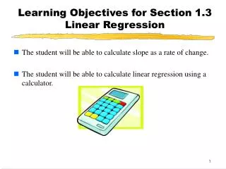
Learning Objectives for Section 1.3 Linear Regression • The student will be able to calculate slope as a rate of change. • The student will be able to calculate linear regression using a calculator.
Mathematical Modeling MATHEMATICAL MODELING is the process of using mathematics to solve real-world problems. This process can be broken down into three steps: • Construct the mathematical model, a problem whose solution will provide information about the real-world problem. • Solve the mathematical model. • Interpret the solution to the mathematical model in terms of the original real-world problem. In this section we will discuss one of the simplest mathematical models, a linear equation.
Slope as a Rate of Change If x and y are related by the equation y = mx +b, where m and b are constants with m not equal to zero, then x and y are linearly related. If (x1, y1) and (x2, y2) are two distinct points on this line, then the slope of the line is This ratio is called the RATE OF CHANGE of y with respect to x.
Slope as a Rate of Change Since the slope of a line is unique, the rate of change of two linearly related variables is constant. Some examples of familiar rates of change are miles per hour and revolutions per minute.
Example 1: Rate of Change • The following linear equation expresses the number of municipal golf courses in the U.S. t years after 1975. • G = 30.8t + 1550 • State the rate of change of the function, and describe what this value signifies within the context of this scenario.
Example 1: Rate of Change (cont.) • The following linear equation expresses the number of municipal golf courses in the U.S. t years after 1975. • G = 30.8t + 1550 • State the vertical intercept of this function, and describe what this value signifies within the context of this scenario.
Linear Regression In real world applications we often encounter numerical data in the form of a table. The powerful mathematical tool, regression analysis, can be used to analyze numerical data. In general, regression analysis is a process for finding a function that best fits a set of data points. In the next example, we use a linear model obtained by using linear regression on a graphing calculator.
Regression Notes Regression: a process used to relate two quantitative variables. • Independent variable: the x variable (or explanatory variable) • Dependent variable: the y variable (or response variable) To interpret the scatterplot, identify the following: • Form • Direction (for linear models) • Strength
Form Form: the function that best describes the relationship between the two variables. Some possible forms would be linear, quadratic, cubic, exponential, or logarithmic.
Direction Direction: a positive or negative direction can be found when looking at linear regression lines only. The direction is found by looking at the sign of the slope.
Strength Strength: how closely the points in the data are gathered around the form.
Making Predictions Predictions should only be made for values of x within the span of the x-values in the data set. Predictions made outside the data set are called extrapolations, which can be dangerous and ridiculous, thus extrapolating is not recommended. To make a prediction within the span of the x-values, hit then . Next, arrow up or down until the regression equation appears in the upper-left hand corner then type in the x-value and hit .
Example of Linear Regression Prices for emerald-shaped diamonds taken from an on-line trader are given in the following table. Find the linear model that best fits this data. Weight (carats) Price 0.5 $1,677 0.6 $2,353 0.7 $2,718 0.8 $3,218 0.9 $3,982
Scatter Plots Enter these values into the lists in a graphing calculator as shown below .
Price of diamond (thousands) Weight (tenths of a carat) Scatter Plots We can plot the data points in the previous example on a Cartesian coordinate plane, either by hand or using a graphing calculator. If we use the calculator, we obtain the following plot:
Example of Linear Regression(continued) Based on the scatterplot, the data appears to be linearly correlated; thus, we can choose linear regression from the statistics menu, we obtain the second screen, which gives the equation of best fit. The linear equation of best fit is y = 5475x - 1042.9.
y = 5475x - 1042.9 Price of emerald (thousands) Weight (tenths of a carat) Scatter Plots We can plot the graph of our line of best fit on top of the scatter plot:
Making a Prediction • Is it appropriate to use the model to predict the price of an emerald-shaped diamond that weighs .75 carats? If so, estimate the price. • Is it appropriate to use the model to predict the price of an emerald-shaped diamond that weighs 2.7 carats? If so, estimate the price.