Download
1 / 29
290 likes | 430 Views
The Seasonality and Partitioning of Atmospheric Heat Transport in a Myriad of Different Climate States. I. Introduction II. A simple energy balance model for the seasonal cycle of energy fluxes III. Dynamical heat transport partitioning

E N D
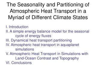
The Seasonality and Partitioning of Atmospheric Heat Transport in a Myriad of Different Climate States I. Introduction II. A simple energy balance model for the seasonal cycle of energy fluxes III. Dynamical heat transport partitioning IV. Atmospheric heat transport in aquaplanet simulations V. Atmospheric Heat Transport in Simulations with Land-Ocean Contrast and Topography VI. Conclusions
Introduction • a. The energy budget framework • b. The dynamical framework • II. A simple energy balance model for the seasonal cycle of energy fluxes • III. Dynamical heat transport partitioning • IV. Atmospheric heat transport in aquaplanet simulations • V. Atmospheric Heat Transport in Simulations with Land-Ocean Contrast and Topography • VI. Conclusions
I. Introduction / a. The energy budget framework 5.7 PW 5.9 PW ERBE DATA
ASR = Absorbed solar SHF = Surface heat flux (-)OLR = Outgoing longwave MHT = Meridional Heat Transp. CTEN = (-) Atmos Column tendency Observed NH I. Introduction / a. The energy budget framework Zonal and Annual Averaged Energy Flux (global mean removed) • All signs defined wrt the atmosphere (e.g., negative OLR is an energy flux deficit for the atmosphere) • Surface heat flux = the total energy flux (radiative plus turbulent) through the surface/atmosphere interface • In the annual mean, positive SHF is equal to oceanic heat flux convergence ERBE/ NCEP
2.2 PW 4.3 PW North Polar Region Tropics 1.4 PW I. Introduction / a. The energy budget framework Annual mean of energy budget poleward of 300N(Departures from global annual mean) Absorbed Solar (ASR) 7.9 PW Surface Heat Flux (SHF) Negative OLR Meridional Heat Transport (MHT)
ASR SHF MHT I. Introduction / a. The energy budget framework Zonal and Seasonal Averaged Energy Flux (zonal, annual average removed) Observed NH (-) OLR CTEN (-) Atmospheric Column tendency ERBE/NCEP DATA
I. Introduction / a. The energy budget framework Seasonal Extratropical Energy Budget
I. Introduction / b. The dynamical framework Transient Eddies (Storm Tracks) Mean Meridional Circulations (MMC) Heat Transport W/m STATIONARY WAVES Temp. Anom. (K) Meridional Wind Anomaly
I. Introduction / b. The dynamical framework Partitioning of heat transport from NCEP reanalysis PW PW PW PW
I. Introduction / b. The dynamical framework Heat transport partitioning at latitude of maximum heat transport
Introduction • II. A simple energy balance model for the seasonal cycle of energy fluxes • III. Dynamical heat transport partitioning • IV. Atmospheric heat transport in aquaplanet simulations • V. Atmospheric Heat Transport in Simulations with Land-Ocean Contrast and Topography • VI. Conclusions
II. A simple energy balance model for the seasonal cycle of energy fluxes OLR’ = BOLR T’A,E ASR’ T’A,E T’A,T BCTENTA,E MHT’ = BMHT(T’A,T – T’A,E) TS’ BOCE TROPICS EXTRATROPICS Primes denote anomaly from global annual mean
II. A simple energy balance model for the seasonal cycle of energy fluxes Annual mean extratropical energy balance • Global mean energy balance requires: OLR’ = 0 or T’T = - T’E = ΔT ASR’ ΔT OLR’ -ΔT MHT’ TROPICS EXTRATROPICS • MHT = BMHT2ΔT • OLR’ = BOLRΔT • MHT / OLR = 2BMHT/BOLR = 2.3 • Real world ratio is 2.6 (including ocean); we shouldn’t be surprised
II. A simple energy balance model for the seasonal cycle of energy fluxes Seasonal cycle of extratropical energy fluxes Asterisks = AGCM simulation Solid = EBM Dotted = theory Based on “B” coefficients • The seasonal amplitude of extratropical energy fluxes is partitioned into ocean storage (SHF), heat transport (MHT), OLR, and atmospheric storage (CTEN) in the approximate ratio: • lSHF’l : lMHT’l : lOLR’l : lCTEN’l ≈ • BOCE : BMHT:BOLR : BCTEN
I. Introduction II. A simple energy balance model for the seasonal cycle of energy fluxes III. Dynamical heat transport partitioning a. Methodology b. Spatial and Temporal patterns of variability IV. Atmospheric heat transport in aquaplanet simulations V. Atmospheric Heat Transport in Simulations with Land-Ocean Contrast and Topography VI. Conclusions
III. Dynamical heat transport partitioning b. Spatial and Temporal patterns of variability ANNUAL MEAN VERTICALLY INTEGRATED HEAT TRANSPORT Transient Eddies Stationary Eddies PW SEASONAL REGRESSION MAP VERTICALLY INTEGRATED HEAT TRANSPORT Transient Eddies Stationary Eddies PW • Units are PW, if the local heat flux existed at all zonal locations • Seasonal regression takes the zonal mean transient or stationary eddy time series at the latitude of maximum heat transport and regresses it against the spatial map • OTHER ANAYLSIS- seasonal eofs, inter-annual eofs, interannual variability
I. Introduction II. A simple energy balance model for the seasonal cycle of energy fluxes III. Dynamical heat transport partitioning IV. Atmospheric heat transport in aquaplanet simulations a.Ocean mixed layer depth experiments b. Longwave emissivity (CO2) experiments c. Planetary rotation rate experiments V. Atmospheric Heat Transport in Simulations with Land-Ocean Contrast and Topography VI. Conclusions
IV. Aquaplanet simulations a. Ocean mixed layer depth experiments METHOD: GFDL 2.1 atmosphere (seasonal insolation) coupled to a slab ocean - Vary mixed ocean depth (Dargan) HYPOTHESIS: Annual mean is unaffected, as the ocean depth increase more seasonal energy goes into ocean storage and the seasonal amplitude of MHT, OLR, and CTEN decrease Asterisks = AGCM simulation Lines = EBM simulations Dotted Lines = B pseudo-steady state theory Donohoe and Battisti 2010
IV. Aquaplanet simulations b. Longwave emissivity (CO2) experiments METHOD: Vary CO2 from LGM (180 ppm) to 4 times PI (1280ppm) [Dargan] HYPOTHESIS: - The efficiency of energy export by longwave radiation (BOLR) goes down, in the annual mean and seasonal cycle the ratio of MHT to OLR decreases (infrared opacity) - The efficiency of MHT (BMHT) increases in a warmer world (more moist transport)
IV. Aquaplanet simulations b. Longwave emissivity (CO2) experiments Annual Mean Heat Transport Heat Transport (PW) Latitude QUAD PI 180 ppm
IV. Aquaplanet simulations c. Planetary Rotation Rates METHOD: Vary Earth’s rotation rate from 0.5X to 2.0X the current rotation rate HYPOTHESIS: With a faster rotation rate, the eddy length scale and efficiency of meridional heat transport (BMHT) will decrease- less heat transport and larger temperature gradient EDDY HEAT TRANSPORT AS A FUNCTION OF Ω [Perpetual Annual Mean Insolation, Realistic Topography] Dry Transient Eddy Heat Transport (1014 W) 0.25 Ω 1.0 Ω (Del Genio and Suozzo 1986) Latitude
I. Introduction II. A simple energy balance model for the seasonal cycle of energy fluxes III. Dynamical heat transport partitioning IV. Atmospheric heat transport in aquaplanet simulations V. Atmospheric Heat Transport in Simulations with Land-Ocean Contrast and Topography a. Land fraction experiments b. Topography experiments c. The full gauntlet (realistic climate states) VI. Conclusions
V. Land-Ocean Contrast and Topography a. Land Fraction Experiments METHOD: A single extratropical continent with North-South Coastlines and varying zonal width – NO TOPOGRAPHY HYPOTHESIS: - ENERGETICS: As land mass increases, more seasonal energy goes into the atmosphere, and the seasonal cycle of heat transport increases - DYNAMICS: Zonal heating anomalies induce stationary waves, heat transport partitioning changes, total heat transport (BMHT)? Solid = EBM simulations Dashed = Pseudo-steady state theory
V. Land-Ocean Contrast and Topography b. Topography experiments --- IDEALIZED METHOD: Aquaplanet with a single idealized mid-latitude topographic feature of varying height, meridional location, and zonal width HYPOTHESIS: - Topography induces stationary wave heat transport - Storm tracks become localized, transient eddy heat transport goes down (seeding?) -Partitioning will change, TOTAL HEAT TRANSPORT? • Dry model, T21 • Newtonian cooling to equilibrium temperature Eddy Heat Transport (K m/s) Equivalently = 0.25 PW (Yu and Hartmann, 1995) Mountain Height (km)
V. Land-Ocean Contrast and Topography b. Topography experiments --- Realistic topography METHOD: Aquaplanet with flat topography, present day topography, and LGM topography (ICE – 5G, Peltier ) HYPOTHESIS: The partitioning between transient and stationary eddies will change– total heat transport? Stationary Eddy DRY Heat Transport Transient Eddy DRY Heat Transport 50 50 LGM -50 -50 Jan Apr Jul Oct Jan Apr Jul Oct 50 50 Latitude MODERN -50 -50 Jan Apr Jul Oct Jan Apr Jul Oct 50 50 MOD - LGM PW PW -50 -50 -2 0 -1 0 1 2 Jan Apr Jul Oct Jan Apr Jul Oct
V. Land-Ocean Contrast and Topography c. The Full Gauntlet (Realistic Climate States) Method: AGCM (CAM3) simulations of LGM, PI, 4XCO2 forced by prescribed SST and sea ice (from CCSM coupled runs), land ice topography, greenhouse gases, and solar insolation Hypothesis: (almost) Everything we’ve learned becomes important: 1. CO2 experiments 2. Land Fraction Experiments (sea ice is like land) 3. Topography 4. Additionally, the absorbed solar radiation changes, we’ll treat this as a forcing (CAMILLE LI)
V. Land-Ocean Contrast and Topography c. The Full Gauntlet (Realistic Climate States)
I. Introduction II. A simple energy balance model for the seasonal cycle of energy fluxes III. Dynamical heat transport partitioning IV. Atmospheric heat transport in aquaplanet simulations V. Atmospheric Heat Transport in Simulations with Land-Ocean Contrast and Topography VI. Conclusions