Download
1 / 55
550 likes | 680 Views
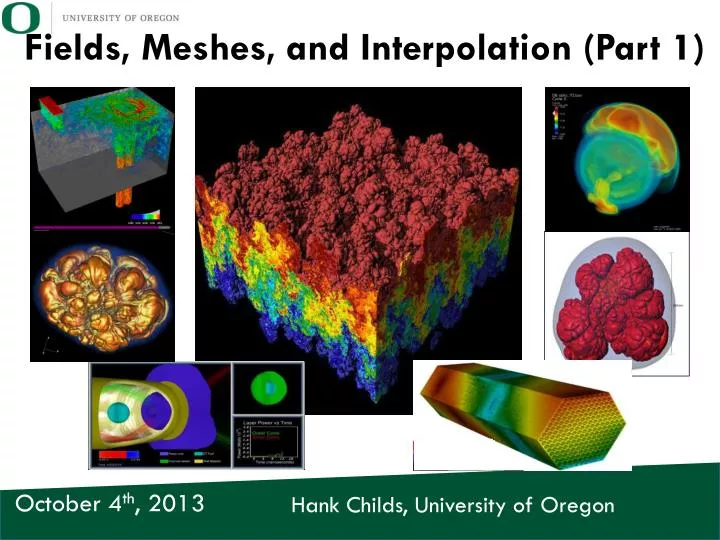
Fields, Meshes, and Interpolation (Part 1). Hank Childs, University of Oregon. October 4 th , 2013. Project #1. Goal: write a specific image Due: “Friday October 4 th ” “6am Saturday October 5 th ” % of grade: 2% Q: Why do I only get 2 days to complete this project?

E N D
Fields, Meshes, and Interpolation (Part1) Hank Childs, University of Oregon October 4th,2013
Project #1 Goal: write a specific image Due: “Friday October 4th” “6am Saturday October 5th” % of grade: 2% Q: Why do I only get 2 days to complete this project? A: We need to need to get multi-platform issues shaken out ASAP. Experience last year was pretty good.
Motivation for today’s lecture • Last class: how visualization works • Many visual metaphors for representing data • How to choose the right tool from the toolbox? • This course: • Describe the tools • Describe the systems that support the tools • This class: we need to understand the data we will be working with before we can talk about the tools • It will go by fast, but you will have the notes and a HW to reinforce it.
Outline Overview Fields Meshes Field interpolation Cell location Project #2
Outline Overview Fields Meshes Field interpolation Cell location Project #2
Elements of a Visualization Legend Provenance Information Reference Cues Display of Data
Elements of a Visualization What is the value at this location? How do you know? What data went into making this picture?
Where does temperature data come from? • Iowa circa 1980s: people phoned in updates What is the temperature along the white line? 6:00pm: Grandma’s friend calls in 82F. 6:00pm: Grandma calls in 80F.
What is the temperature at points between Ralston and Glidden? 82F Temperature 81F 80F ~ ~ D=0, Ralston, IA D=10 miles, Glidden, IA Distance
Ways Visualization Can Lie Visualization Errors: Illusion of certainty Poor choices of parameters Visualization Program Data Errors: Data collection is inaccurate Data collected too sparsely
Outline Overview Fields Meshes Field interpolation Cell location Project #2
Fields & Spaces • Fields are defined over “spaces”. • We will be considering 2D & 3D spaces. • Defined by an origin and three vectors (or two vectors) that define orientation.
Scalar Fields The temperature at 41.2324° N, 98.4160° W is 66F. • Defined: associate a scalar with every point in space. • What is a scalar? • A: a real number • Examples: • Temperature • Density • Pressure Fields are defined at every location in a space (example space: USA)
Vector Fields The velocity at location (5, 6) is (-0.1, -1) The velocity at location (10, 5) is (-0.2, 1.5) • Defined: associate a vector with every point in space. • What is a vector? • A: a direction and a magnitude • Examples: • Velocity Typically, 2D spaces have 2 components in their vector field, and 3D spaces have 3 components in their vector field.
Vector Fields Representing dense data is hard and requires special techniques.
More fields (discussed later in course) • Tensor fields • Functions • Volume fractions • Multi-variate data
Outline Overview Fields Meshes Field interpolation Cell location Project #2
Mesh What we want
An example mesh Where is the data on this mesh? (for today, it is at the vertices of the triangles)
An example mesh Why do you think the triangles change size?
Anatomy of a computational mesh • Meshes contain: • Cells • Points • This mesh contains 3 cells and 13 vertices • Pseudonyms: • Cell == Element == Zone • Point == Vertex == Node
Types of Meshes Adaptive Mesh Refinement Curvilinear Unstructured We will discuss all of these mesh types more later in the course.
Rectilinear meshes • Rectilinear meshes are easy and compact to specify: • Locations of X positions • Locations of Y positions • 3D: locations of Z positions • Then: mesh vertices are at the cross product. • Example: • X={0,1,2,3} • Y={2,3,5,6} Y=6 Y=5 Y=3 Y=2 X=0 X=1 X=2 X=3
Rectilinear meshes aren’t just the easiest to deal with … they are also very common
Quiz Time • A 3D rectilinear mesh has: • X = {1, 3, 5, 7, 9} • Y = {2, 3, 5, 7, 11, 13, 17} • Z = {1, 2, 3, 5, 8, 13, 21, 34, 55} • How many points? • How many cells? = 5*7*9 = 315 Y=6 = 4*6*8 = 192 Y=5 Y=3 Y=2 X=0 X=1 X=2 X=3
Definition: dimensions • A 3D rectilinear mesh has: • X = {1, 3, 5, 7, 9} • Y = {2, 3, 5, 7, 11, 13, 17} • Z = {1, 2, 3, 5, 8, 13, 21, 34, 55} • Then its dimensions are 5x7x9
How to Index Points • Motivation: many algorithms need to iterate over points. for (inti = 0 ; i < numPoints ;i++) { double *pt = GetPoint(i); AnalyzePoint(pt); }
Schemes for indexing points Point indices Logical point indices What would these indices be good for?
How to Index Points • Problem description: define a bijective function, F, between two sets: • Set 1: {(i,j,k): 0<=i<nX, 0<=j<nY, 0<=k<nZ} • Set 2: {0, 1, …, nPoints-1} • Set 1 is called “logical indices” • Set 2 is called “point indices” Note: for the rest of this presentation, we will focus on 2D rectilinear meshes.
How to Index Points • Many possible conventions for indexing points and cells. • Most common variants: • X-axis varies most quickly • X-axis varies most slowly F
Bijective function for rectilinear meshes for this course intGetPoint(inti, int j, intnX, intnY) { return j*nX + i; } F
Bijective function for rectilinear meshes for this course int *GetLogicalPointIndex(int point, intnX, intnY) { intrv[2]; rv[0] = point % nX; rv[1] = (point/nX); return rv; // terrible code!! }
int *GetLogicalPointIndex(int point, intnX, intnY) { intrv[2]; rv[0] = point % nX; rv[1] = (point/nX); return rv; } F
Quiz Time #2 • A mesh has dimensions 6x8. • What is the point index for (3,7)? • What are the logical indices for point 37? = 45 = (1,6) int *GetLogicalPointIndex(int point, intnX, intnY) { intrv[2]; rv[0] = point % nX; rv[1] = (point/nX); return rv; // terrible code!! } intGetPoint(inti, int j, intnX, intnY) { return j*nX + i; }
Quiz Time #3 • A vector field is defined on a mesh with dimensions 100x100 • The vector field is defined with double precision data. • How many bytes to store this data? = 100x100x2x8 = 160,000
Bijective function for rectilinear meshes for this course intGetCell(inti, int j intnX, intnY) { return j*(nX-1) + i; }
Bijective function for rectilinear meshes for this course int *GetLogicalCellIndex(intcell, intnX, intnY) { intrv[2]; rv[0] = cell % (nX-1); rv[1] = (cell/(nX-1)); return rv; // terrible code!! }
Outline Overview Fields Meshes Field interpolation Cell location Project #2
Linear Interpolation for Scalar Field F Goal: have data at some points & want to interpolate data to any location
Linear Interpolation for Scalar Field F F(A) F(X) F(B) X A B
Linear Interpolation for Scalar Field F F(A) F(X) F(B) X A B • General equation to interpolate: • F(X) = F(A) + t*(F(B)-F(A)) • t is proportion of X between A and B • t = (X-A)/(B-A)
Quiz Time #4 • F(3) = 5, F(6) = 11 • What is F(4)? = 5 + (4-3)/(6-3)*(11-5) = 7 • General equation to interpolate: • F(X) = F(A) + t*(F(B)-F(A)) • t is proportion of X between A and B • t = (X-A)/(B-A)
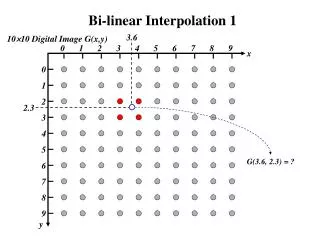
Bilinear interpolation for Scalar Field F F(1,1) = 6 F(0,1) = 1 Idea: we know how to interpolate along lines. Let’s keep doing that and work our way to the middle. What is value of F(0.3, 0.4)? F(0.3, 0) = 8.5 F(0.3, 1) = 2.5 = 6.1 F(0,0) = 10 F(1,0) = 5 • General equation to interpolate: F(X) = F(A) + t*(F(B)-F(A))
Outline Overview Fields Meshes Field interpolation Cell location Project #2
Cell location • Problem definition: you have a physical location (P). You want to identify which cell contains P. • Solution: multiple approaches that incorporate spatial data structures. • Best data structure depends on nature of input data. • More on this later in the quarter.
Cell location for project 2 • Traverse X and Y arrays and find the logical cell index. • X={0, 0.05, 0.1, 0.15, 0.2, 0.25} • Y={0, 0.05, 0.1, 0.15, 0.2, 0.25} • (Quiz) what cell contains (0.17,0.08)? = (3,1)
Facts about cell (3,1) • It’s cell index is 8. • It contains points (3,1), (4,1), (3,2), and (4,2). • Facts about point (3,1): • It’s location is (X[3], Y[1]) • It’s point index is 9. • It’s scalar value is F(9). • Similar facts for other points. • we have enough info to do bilinear interpolation
Outline Overview Fields Meshes Field interpolation Cell location Project #2
Project 2: Field evaluation • Goal: for point P, find F(P) • Strategy in a nut shell: • Find cell C that contains P • Find C’s 4 vertices, V0, V1, V2, and V3 • Find F(V0), F(V1), F(V2), and F(V3) • Find locations of V0, V1, V2, and V3 • Perform bilinear interpolation to location P