Download
1 / 41
410 likes | 769 Views
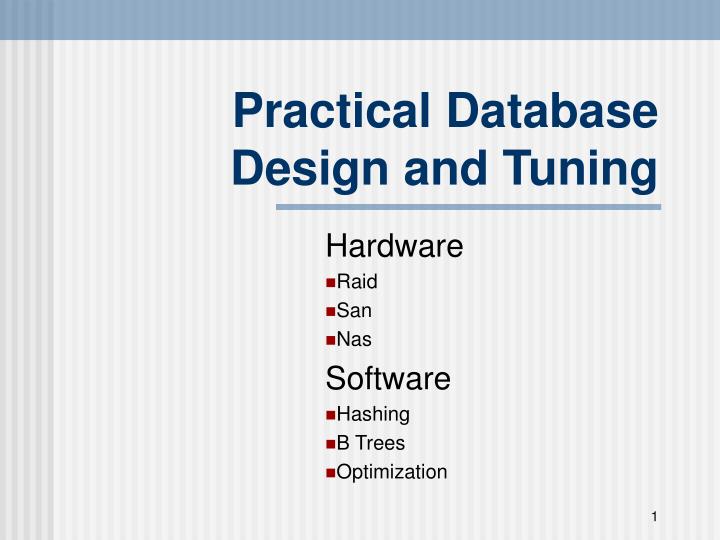
Practical Database Design and Tuning. Hardware Raid San Nas Software Hashing B Trees Optimization . Disk Storage Devices. Parallelizing Disk Access using RAID Technology. Secondary storage technology must take steps to keep up in performance and reliability with processor technology.

E N D
Practical Database Design and Tuning Hardware Raid San Nas Software Hashing B Trees Optimization
Parallelizing Disk Access using RAID Technology. • Secondary storage technology must take steps to keep up in performance and reliability with processor technology. • A major advance in secondary storage technology is represented by the development of RAID, which originally stood for Redundant Arrays of Inexpensive Disks. • The main goal of RAID is to even out the widely different rates of performance improvement of disks against those in memory and microprocessors.
RAID Technology (cont.) • A natural solution is a large array of small independent disks acting as a single higher-performance logical disk. A concept called data striping is used, which utilizes parallelism to improve disk performance. • Data striping distributes data transparently over multiple disks to make them appear as a single large, fast disk.
RAID Technology (cont.) Different raid organizations were defined based on different combinations of the two factors of granularity of data interleaving (striping) and pattern used to compute redundant information. • Raid level 0 has no redundant data and hence has the best write performance. • Raid level 1 uses mirrored disks. • Raid level 2 uses memory-style redundancy by using Hamming codes, which contain parity bits for distinct overlapping subsets of components. Level 2 includes both error detection and correction. • Raid level 3 uses a single parity disk relying on the disk controller to figure out which disk has failed. • Raid Levels 4 and 5 use block-level data striping, with level 5 distributing data and parity information across all disks. • Raid level 6 applies the so-called P + Q redundancy scheme using Reed-Soloman codes to protect against up to two disk failures by using just two redundant disks.
Use of RAID Technology (cont.) Different raid organizations are being used under different situations • Raid level 1 (mirrored disks)is the easiest for rebuild of a disk from other disks • It is used for critical applications like logs • Raid level 2 uses memory-style redundancy by using Hamming codes, which contain parity bits for distinct overlapping subsets of components. Level 2 includes both error detection and correction. • Raid level 3 ( single parity disks relying on the disk controller to figure out which disk has failed) and level 5 (block-level data striping) are preferred for Large volume storage, with level 3 giving higher transfer rates. • Most popular uses of the RAID technology currently are: Level 0 (with striping), Level 1 (with mirroring) and Level 5 with an extra drive for parity. • Design Decisions for RAID include – level of RAID, number of disks, choice of parity schemes, and grouping of disks for block-level striping.
Storage Area Networks • The demand for higher storage has risen considerably in recent times. • Organizations have a need to move from a static fixed data center oriented operation to a more flexible and dynamic infrastructure for information processing. • Thus they are moving to a concept of Storage Area Networks (SANs). In a SAN, online storage peripherals are configured as nodes on a high-speed network and can be attached and detached from servers in a very flexible manner. • This allows storage systems to be placed at longer distances from the servers and provide different performance and connectivity options.
Storage Area Networks (contd.) Advantages of SANs are: • Flexible many-to-many connectivity among servers and storage devices using fiber channel hubs and switches. • Up to 10km separation between a server and a storage system using appropriate fiber optic cables. • Better isolation capabilities allowing nondisruptive addition of new peripherals and servers. • SANs face the problem of combining storage options from multiple vendors and dealing with evolving standards of storage management software and hardware.
NAS (Network Attached Storage) • Network-attached storage (NAS) systems are generally computing-storage devices that can be accessed over a computer network (usually TCP/IP), rather than directly being connected to the computer (via a computer bus such as SCSI). This enables multiple computers to share the same storage space at once, which minimizes overhead by centrally managing hard disks. NAS systems usually contain one or more hard disks, often arranged into logical, redundant storage containers or RAID arrays.The protocol used with NAS is a file based protocol such as NFS, Samba or Microsoft's Common Internet File System (CIFS). In reality, there is a miniature operating system on the device such as Celerra on EMC's devices or NetOS on NetApp NAS devices.
Hashed Files • The term "hash" apparently comes by way of analogy with its standard meaning in the physical world, to "chop and mix." Knuth notes that Hans Peter Luhn of IBM appears to have been the first to use the concept, in a memo dated January 1953; the term hash came into use some ten years later.
Hashed Files • Hashing for disk files is called External Hashing • The file blocks are divided into M equal-sized buckets, numbered bucket0, bucket1, ..., bucket M-1. Typically, a bucket corresponds to one (or a fixed number of) disk block. • One of the file fields is designated to be the hash key of the file. • The record with hash key value K is stored in bucket i, where i=h(K), and h is the hashing function. • Search is very efficient on the hash key. • Collisions occur when a new record hashes to a bucket that is already full. An overflow file is kept for storing such records. Overflow records that hash to each bucket can be linked together.
Hashed Files (cont.) There are numerous methods for collision resolution, including the following: • Open addressing: Proceeding from the occupied position specified by the hash address, the program checks the subsequent positions in order until an unused (empty) position is found. • Chaining: For this method, various overflow locations are kept, usually by extending the array with a number of overflow positions. In addition, a pointer field is added to each record location. A collision is resolved by placing the new record in an unused overflow location and setting the pointer of the occupied hash address location to the address of that overflow location. • Multiple hashing(Rehash): The program applies a second hash function if the first results in a collision. If another collision results, the program uses open addressing or applies a third hash function and then uses open addressing if necessary.
Hashed Files (cont.) • To reduce overflow records, a hash file is typically kept 70-80% full. • The hash function h should distribute the records uniformly among the buckets; otherwise, search time will be increased because many overflow records will exist (Test a Sample data ) • Main disadvantages of static external hashing: - Fixed number of buckets M is a problem if the number of records in the file grows or shrinks. - Ordered access on the hash key is quite inefficient (requires sorting the records).
Dynamic And Extendible Hashed Files Dynamic and Extendible Hashing Techniques • Hashing techniques are adapted to allow the dynamic growth and shrinking of the number of file records. • These techniques include the following: dynamic hashing , extendible hashing , and linear hashing . • Both dynamic and extendible hashing use the binary representation of the hash value h(K) in order to access a directory. In dynamic hashing the directory is a binary tree. In extendible hashing the directory is an array of size 2d where d is called the global depth.
Dynamic And Extendible Hashing • The directories can be stored on disk, and they expand or shrink dynamically. Directory entries point to the disk blocks that contain the stored records. • An insertion in a disk block that is full causes the block to split into two blocks and the records are redistributed among the two blocks. The directory is updated appropriately. • Dynamic and extendible hashing do not require an overflow area. • Linear hashing does require an overflow area but does not use a directory. Blocks are split in linear order as the file expands.
Dynamic Multilevel Indexes Using B-Trees and B+-Trees • The B-tree's creator, Rudolf Bayer, has not explained what the B stands for. The most common belief is that B stands for balanced, as all the leaf nodes are at the same level in the tree. B may also stand for Bayer, or for Boeing, because he was working for Boeing Scientific Research Labs. • Rudolf Bayer has been Professor (emeritus) of Informatics at the Technical University of Munich since 1972. He is famous for inventing the data sorting structures the B-tree with Edward M. McCreight, and later the UB-tree with Volker Markl.He is a recipient of 2001ACMSIGMODEdgar F. Codd Innovations Award.
Dynamic Multilevel Indexes Using B-Trees and B+-Trees • Because of the insertion and deletion problem, most multi-level indexes use B-tree or B+-tree data structures, which leave space in each tree node (disk block) to allow for new index entries • These data structures are variations of search trees that allow efficient insertion and deletion of new search values. • In B-Tree and B+-Tree data structures, each node corresponds to a disk block • Each node is kept between half-full and completely full
Dynamic Multilevel Indexes Using B-Trees and B+-Trees • An insertion into a node that is not full is quite efficient; if a node is full the insertion causes a split into two nodes • Splitting may propagate to other tree levels • A deletion is quite efficient if a node does not become less than half full • If a deletion causes a node to become less than half full, it must be merged with neighboring nodes
Difference between B-tree and B+-tree • In a B-tree, pointers to data records exist at all levels of the tree • In a B+-tree, all pointers to data records exists at the leaf-level nodes • A B+-tree can have less levels (or higher capacity of search values) than the corresponding B-tree
B-tree structures. (a) A node in a B-tree with q – 1 search values. (b) A B-tree of order p = 3. The values were inserted in the order 8, 5, 1, 7, 3, 12, 9, 6.
The nodes of a B+-tree. (a) Internal node of a B+-tree with q –1 search values. (b) Leaf node of a B+-tree with q – 1 search values and q – 1 data pointers.
An example of insertion in a B+-tree with q = 3 and pleaf = 2.
1. Translating SQL Queries into Relational Algebra • Query block: the basic unit that can be translated into the algebraic operators and optimized. • A query block contains a single SELECT-FROM-WHERE expression, as well as GROUP BY and HAVING clause if these are part of the block. • Nested queries within a query are identified as separate query blocks. • Aggregate operators in SQL must be included in the extended algebra.
Algorithms for SELECT and JOIN Operations Implementing the SELECT Operation (cont.): Search Methods for Simple Selection: • S1. Linear search (brute force): Retrieve every record in the file, and test whether its attribute values satisfy the selection condition. • S2. Binary search: If the selection condition involves an equality comparison on a key attribute on which the file is ordered, binary search (which is more efficient than linear search) can be used. (See OP1). • S3. Using a primary index or hash key to retrieve a single record: If the selection condition involves an equality comparison on a key attribute with a primary index (or a hash key), use the primary index (or the hash key) to retrieve the record.
Algorithms for SELECT and JOIN Operations Implementing the JOIN Operation • Factors affecting JOIN performance • Available buffer space • Join selection factor • Choice of inner VS outer relation Use Common Sense First do the WHERE conditions in the various tables and then do the JOIN Use DISTINCT if possible before the join In the FROM statement think about the order to select the tables, it might make it faster
Query Optimization Cost Components for Query Execution • Access cost to secondary storage • Storage cost • Computation cost • Memory usage cost • Communication cost
Physical Database Design in Relational Databases Factors that Influence Physical Database Design Analyzing the database queries and transactions For each query, the following information is needed. • The files that will be accessed by the query; • The attributes on which any selection conditions for the query are specified; • The attributes on which any join conditions or conditions to link multiple tables or objects for the query are specified; • The attributes whose values will be retrieved by the query.
Physical Database Design in Relational Databases(3) Factors that Influence Physical Database Design (cont.) Analyzing the expected frequency of invocation of queries and transactions • The expected frequency information, along with the attribute information collected on each query and transaction, is used to compile a cumulative list of expected frequency of use for all the queries and transactions. • It is expressed as the expected frequency of using each attribute in each file as a selection attribute or join attribute, over all the queries and transactions. • Pareto’s 80-20 rule: 20 % queries are made 80 % of the time
Physical Database Design in Relational Databases Physical Database Design Decisions • Design decisions about indexing • Whether to index an attribute? • What attribute or attributes to index on? • Whether to set up a clustered index? • Whether to use a hash index over a tree index? • Whether to use dynamic hashing for the file?
An Overview of Database Tuning in Relational Systems • Tuning: the process of continuing to revise/adjust the physical database design by monitoring resource utilization as well as internal DBMS processing to reveal bottlenecks such as contention for the same data or devices. • Goal: • To make application run faster • To lower the response time of queries/transactions • To improve the overall throughput of transactions
Statistics internally collected in DBMSs: Size of individual tables Number of distinct values in a column The number of times a particular query or transaction is submitted/executed in an interval of time The times required for different phases of query and transaction processing Statistics obtained from monitoring: Storage statistics I/O and device performance statistics Query/transaction processing statistics Locking/logging related statistics Index statistics Know your Data (sample size it)
An Overview of Database Tuning in Relational Systems Tuning Indexes • Reasons to tuning indexes • Certain queries may take too long to run for lack of an index; • Certain indexes may not get utilized at all; • Certain indexes may be causing excessive overhead because the index is on an attribute that undergoes frequent changes • Options to tuning indexes • Drop or/and build new indexes • Change a non-clustered index to a clustered index (and vice versa) • Rebuilding the index
An Overview of Database Tuning in Relational Systems (7) Tuning Queries • Indications for tuning queries • A query issues too many disk accesses • The query plan shows that relevant indexes are not being used. • Typical instances for query tuning • Many query optimizers do not use indexes in the presence of arithmetic expressions, numerical comparisons of attributes of different sizes and precision, NULL comparisons, and sub-string comparisons. • Indexes are often not used for nested queries using IN;