Download

1 / 28
290 likes | 429 Views
Lecture 09 Segmentation ( ch 8 ) ch. 8 of Machine Vision by Wesley E. Snyder & Hairong Qi. Spring 2012 BioE 2630 (Pitt) : 16-725 (CMU RI) 18-791 (CMU ECE) : 42-735 (CMU BME) Dr. John Galeotti. Segmentation. There is room for interpretation here…. A partitioning…

E N D
Lecture 09Segmentation (ch 8)ch.8 of Machine Vision by Wesley E. Snyder & Hairong Qi Spring 2012 BioE2630 (Pitt) : 16-725 (CMU RI) 18-791 (CMU ECE) : 42-735 (CMU BME) Dr. John Galeotti
Segmentation There is room for interpretation here… • A partitioning… • Into connected regions… • Where each region is: • Homogeneous • Identified by a unique label And here
The “big picture:” Examples from The ITK Software Guide Figures 9.12 (top) & 9.1 (bottom) from the ITK Software Guide v 2.4, by Luis Ibáñez, et al.
Connected Regions • Lots of room for interpretation • Possible meanings: • In an image • Don’t forget about the connectivity paradox • In “real life” • How do you measure that from an image? • Background vs. foreground • This image has 2 foreground regions • But is has 4 connected components
Homogeneous Regions • Lots of room for interpretation • Possible meanings: • All pixels are the “same”brightness • Close to some representative (mean) brightness • Color • Motion • Texture • Generically & formally: • The values of each pixel are consistent with having been generated by a particular model (such as a probability distribution)
Segmentation Methods • There are many methods • Here are a few examples: • Threshold-based • Guaranteed to form closed regions (why?) • Region-based • Start with elemental homogonous regions • Merge & split them • Hybrid methods • E.g., watershed
Human Segmentation • Class discussion: • How do humans segment what they see? • What about a static image? • How do radiologists segment a medical image? • Is human segmentation task-dependent? • So, how would you compare the accuracy of one segmentation to another?
Segmentation by Thresholding • Results in a binary labeling • When would we want this? • When not? • Notion of object(s)/foreground vs. background We want to segment a single object… Or the single set of all objects of a given type Any time we need to distinguish between multiple objects
Segmentation by Thresholding • Real-world annoyances: • Most images are not taken under perfectly uniform illumination (or radiation, contrast agent, etc.) • Optical imaging devices are typically not equally sensitive across their field of view (vignetting, etc.) • These are less problematic for most radiological images than for camera images, ultrasound, OCT, etc. • Problem: The same object often has different intensities at different locations in an image • Solution: Use local thresholds
Local Thresholding • Typically, block thresholding: • Tessellate the image into rectangular blocks • Use different threshold parameter(s) for each block • Slower (but better?): • Use a moving window
Computing Thresholds • In a few lucky cases: • If multiple, similar objects will be imaged under virtually identical conditions, then… • Carefully choose a good threshold (often by hand) for the first object, and then… • Use that threshold for all future objects • Remember, we may be doing this for each block in the image
Computing Thresholds • Most of the time: • If we expect to see different objects under different conditions, then… • We need to automate the selection of thresholds • Many ways to do this • Remember, we may be doing this for each block in the image
Computing Thresholds • If we expect lots of contrast, then use: • Tmin = iavg + OR Tmax = iavg - • More typically: • Histogram analysis 80 pixels with an intensity of 20 96 pixels with an intensity of 100
Histogram analysis • Idea: Choose a threshold between the peaks • Histograms often require pre-processing • How to find the peaks? • Try fitting Gaussians to the histogram • Use their intersection(s) as the threshold(s) • See the text for details • How many Gaussians to try to fit? This lobe requires Tmin andTmax Requires prior knowledge!
Connected Component Analysis • Recall that thresholding produces a binary segmentation. • What if thresholding detects multiple objects, and we need to analyze each of them separately? • Multiple bones in a CT scan • Multiple fiducial markers • Etc. • We want a way to give a different label to each detected object
Connected Component Analysis • What separates one thresholded object from another one? • Space! • More precisely, background pixels • Two objects are separate if they are not connected by foreground pixels • Connected component analysis lets us: • Assign a different label to each (disconnected) object… • from the (binary) set of segmented objects
Connected Component Analysis • Graph-theory basis • Example containing 2 (foreground) connected components • Thresholding gives us the top figure • Connected Component Analysis on the foreground of the top figure gives us the bottom figure Thresholding Thresholding + Connected Component Analysis of Foreground
Connected Component Analysis • Example of a label image: • A label image L is isomorphic to its original image f • (pixel-by-pixel correspondence) • Each component is given its own numerical label N Label image
Assume: A threshold segmentation already marked object pixels as black in f • Find an unlabeled black pixel; that is, L(x, y) = 0 . Choose a new label number for this region, call it N . If all pixels have been labeled, stop. • L(x, y) N • Push unlabeled neighboring object pixels onto the stack • If f(x-1, y) is black and L(x-1, y) = 0 , push (x-1, y) onto the stack. • If f(x+1, y) is black and L(x+1, y) = 0 , push (x+1, y) onto the stack. • If f(x, y-1) is black and L(x, y-1) = 0 , push (x, y-1) onto the stack. • If f(x, y+1) is black and L(x, y+1) = 0 , push (x, y+1) onto the stack. • Choose an new (x, y) by popping the stack. • If the stack is empty, go to 1, else go to 2. { Flood-fill Recursive Region Growing • One method of doing connected component analysis • Basically a series of recursive flood-fills
Trees Instead of Label Images for Scale Space • Normal practice: Label image identifies which pixels belong to which regions. • Tree-based approach: • A graph is established • Each node segmented object • Levels of the graph correspond to levels of scale • A “parent node” is at a higher (more blurred) level of scale than the children of that node. • All the children of a given parent are assumed to lie in the same region. • A child node is related to a parent if: • It is geometrically close to the parent, and • It is similar in intensity
Texture Segmentation • Two fundamentally different types of textures: • Deterministic • Pattern replications • E.g. brick wall or a grid of ceiling tiles • Use template matching, or • Use FT to find spatial frequencies • Random • E.g. the pattern on a single cinder block or a single ceiling tile • Model with Markov random fields • Remember: • Ultimately, you need a single number with which to compare a pixel to a neighbor
Salient points Segmentation of Curves • Assume: The object is already segmented • We have a curve tracing around an object • New problem: Segment the curve • Identify “salient” points along the boundary • Salient points in curve ≈ edges in image • Enables characterizing the curve between the salient points. • Can fit a “reasonable” low order curve between 2 salient points
The Nature of Curves • A curve is a 1D function, which is simply bent in (“lives in”) ND space. • That is, a curve can be parameterized using a single parameter (hence, 1D). • The parameter is usually arc length, s • Even though not invariant to affine transforms.
The Nature of Curves • The speed of a curve at a point s is: • Denote the outward normal direction at point s as n(s) • Suppose the curve is closed: • The concepts of INSIDE and OUTSIDE make sense • Given a point x = [xi,yi] not on the curve, • Let x represent the closest point on the curve to x • The arc length at x is defined to be sx. • x is INSIDE the curve if: [x - x] n(sx) 0 • And OUTSIDE otherwise.
Segmentation of Surfaces • A surface is a 2D function, which is simply bent in (“lives in”) three-space. • 2 philosophies: • Seek surfaces which do not bend too quickly • Segment regions along lines of high surface curvature (fitting a surface with a set of planes) • Points where planes meet produce either “roof” edges or “step” edges, depending on viewpoint • Assume some equation • E.g. a quadric (a general second order surface) • All points which satisfy the equation and which are adjacent belong to the same surface. The “difference” in edges is only from viewpoint. But curvature is invariant to viewpoint! (Unfortunately, curvature is sensitive to noise.)
Describing Surfaces • An explicit representation might be: • An implicit form is: • The latter is a quadric: • A general form • Describes all second order surfaces (cones, spheres, planes, ellipsoids, etc.) • Can’t linearly solve an explicit quadric for the vector of coefficients (to fit to data) • You would have a √on the right hand side!
Fitting an Implicit Quadric • Define • Then: • We have a parameter vector • q = [a,b,c,d,e,f,g,h,i,j]T • If the point [xi,yi,zi]T is on the surface described by q, • Then f(xi,yi,zi) should = 0. • Define a level set of a function as the collection of points [xi,yi,zi]T such that f(xi,yi,zi)=L for some scalar constant L. • Solve for q by minimizing the distances between every point, [xi,yi,zi]T, and the surface described by q, which is f(xi,yi,zi)=0.
Final Notes • Next class: Active contours! • Shadow Program!