Download
1 / 54
540 likes | 685 Views
Seasonal Unit Root Tests in Long Periodicity Cases. D. A. Dickey Ying Zhang.

E N D
Seasonal Unit Root Tests in Long Periodicity Cases D. A. Dickey Ying Zhang
Natural gas-a colorless, odorless, gaseous hydrocarbon-may be stored in a number of different ways. It is most commonly held in inventory underground under pressure in three types of facilities. These are: (1) depleted reservoirs in oil and/or gas fields, (2) aquifers, and (3) salt cavern formations. (Natural gas is also stored in liquid form in above-ground tanks).
1. Regression with Time Series Errors • Y(t) = a + bt + seasonal effects + Z(t), • Z(t) a stationary time series • Seasonal effects: • Sinusoids, • Seasonal dummy variables • 2. Dynamic Seasonal Models • Y(t) = Y(t-d) + e(t) copy of last season • Y(t) = Y(t-d) + e(t) – b e(t-d) EWMA of past seasons • Y(t) = Y(t-1) + [Y(t-d)-Y(t-d-1)] + Z(t) • Z(t) = e(t) PROC CUT&PASTE; • Z(t) = e(t) – a e(t-1) – b e(t-d) + ab e(t-d-1) “airline” • Z(t) = (1-aB)(1-bBd) e(t)
Summary: • Both models can give same predictions for pure trend + seasonal functions. • For data, lag model looks back 1 year and ignores (or discounts) others. Good for slowly changing seasonality. • For data, dummy variable model weights all years equally. Good for very regular seasonality. • 4. Differences in forecast errors too!
A general seasonal model: Yt –f(t) = r(Yt-d –f(t-d)) + et f(t) = deterministic components H0: r=1 Under H0, period d functions annihilated. f periodic Yt –Yt-d = (r-1)(Yt-d –f(t-d)) + et r=1 Yt –Yt-d = et
Use double subscripts: Quarterly (d=4) example, m years, f(t)=0
Numerator is Denominator is Known unit root facts (s2=1): (1) Moments (d=1 case or individual terms) E{Ns} = 0, E{Ds} = (m-1)/(2m)1/2 Var{Ns} = (m-1)/(2m)1/2 Var{Ds} = (m-1)(m2-m+1)/(3m3)1/3 Cov{Ns, Ds} = (m-1)(m-2)/(3m2) 1/3 (2) Studentized statistic asymptotically equivalent to (numerator sum) / (denominator sum)1/2
Basic idea is simple: Large d numerator approximately normal Large d denominator converges to E{denominator}
Nice proof Grandpa! As you see, I’m very excited.
CDFs d=4 tand N(0,1) -1.645 0 1.645 (SAS)
CDFs d=4 md1/2(r-1) and N(0,2) -2.386 0 2.386
Improving the Normal Approximation: JASA paper (Dickey, Hasza, Fuller, 1984 ) gives limit distribution for studentized statistic (d=12) 5th %ile = -1.80 95th %ile = 1.52 50th %ile: -0.14 (Note: (1.52-1.80)/2 = -0.14 !!) Difference: 1.52+1.80 = 3.32, 2(1.645) = 3.29 (close !!) Suggestion: shift by median CLT limit distribution median is 0.
Median as function of seasonality d: 1. Get medians for d=2, 4,12 from DHF 2. Plot median vs. d-1/2 (d=2,4,12,limit)
Median as function of seasonality d: Regress median on d-1/2 Slope very close to ½, Intercept very close to 0. Median Shifts and Tau Percentiles. d med -1/(2 ) p01 p025 p05 p10 2 -0.35 -0.35355 -2.67990 -2.31352 -1.99841 -1.63510 4 -0.24 -0.25000 -2.57635 -2.20996 -1.89485 -1.53155 12 -0.14 -0.14434 -2.47069 -2.10430 -1.78919 -1.42589 inf 0.00 0 -2.32685 -1.96046 -1.64535 -1.28205
Simulation Evidence • m= 100, various d values • 2 sets of 40,000 t statistics at each (m,d) • e.g. d=365 and m=100, (daily data 100 years) • 36500x40000 = 1.46 billion generated data points. • SAS: only 10 minutes run time ! • Overlay percentiles (adjusted t) on N(0,1) • Duplicates almost exactly the same.
Simulation Evidence - Detrending • m= 20, d =4, 6, 12, 24, 52, 96, 168, 365 • 96 quarter hours/day, 168 hours/week • Detrending: • None • Constant, linear, quadratic • Period d sinusoids (fundamental & harmonic) • Sets of 20,000 t statistics at each (m,d).
Standard tau percentiles for various adjustments Three replicates (of 20,000) per d value Conclusions: Spread between percentiles about constant (and close to N(0,1) spread) Medians smooth function of 1/sqrt(d) Degree of detrending matters Cubic smoothing regression plotted with raw %iles.
Claim: As d infinity, Tau N(0,1) for all of these forms of detrending Seasonal random walk Z, data Y. Y = Xb + Z Detrend by OLS: Seasonal Random Walk has d “channels” of m values Denominator is sum of d quadratic forms Without detrending each has eigenvalues can be written as
k = rank of X matrix Middle matrix is diagonal. Projection => k diagonal entries 1 rest 0 Denominator quadratic form contains k times maximum eigenvalue = O(km2) Upper probability bound on unnormalized quadratic form. Normalization is m2d so k/d0 suffices for no limit effect of detrending. Same for numerator, estimator, tau statistic.
Based on Taylor series (for large m) adjustment is for regression adjustments with k columns selected from intercept and Fourier sines and cosines.
Your talk seems better now Grandpa!
Allowing for augmenting terms, as in seasonal multiplicative model, follows the same proof as in DHF. Natural gas data: Procedure (1) Compute residuals (trend + harmonics) (2) AR(2) fit to span 52 differences of residuals (3) Filter with AR(2) Ft = filtered series Wt = span 52 differences Ft – Ft-52 (4) Regress Wt on Ft-52 Wt-1 Wt-2
The REG Procedure Dependent Variable: Diff Sum of Mean Source DF Squares Square F Value Pr > F Model 3 718362 239454 231.53 <.0001 Error 679 702233 1034.21632 Corrected Total 682 1420595 Parameter Estimates Parameter Standard Variable DF Estimate Error t Value Pr > |t| Intercept 1 -0.68125 1.23111 -0.55 0.5802 L52FY 1 -0.99746 0.03800 -26.25 <.0001 Diff1 1 0.01417 0.00777 1.82 0.0686 Diff2 1 -0.01152 0.00730 -1.58 0.1151
Follow up: Lag 52 coefficient near -1 suggests a52-1 near -1 Perhaps no lag correlation in the presence of sinusoids Fit ARIMAX model as a check (AR(2), no seasonal lag): Standard Approx Parameter Estimate Error t Value Pr > |t| Lag Variable MU 727.58194 684.44164 1.06 0.2878 0 total AR1,1 1.37442 0.03379 40.67 <.0001 1 total AR1,2 -0.38964 0.03381 -11.53 <.0001 2 total NUM1 0.09520 0.04525 2.10 0.0354 0 date NUM2 -883.25146 23.18237 -38.10 <.0001 0 s1 NUM3 240.92573 23.05715 10.45 <.0001 0 c1 NUM4 -133.27021 11.51098 -11.58 <.0001 0 s2 NUM5 122.42419 11.53277 10.62 <.0001 0 c2
Lack of fit? Box-Ljung test on residuals Autocorrelation Check of Residuals To Chi- Pr > Lag Square DF ChiSq -------------Autocorrelations------------ 6 1.40 4 0.8449 0.008 -0.012 0.001 -0.000 -0.023 0.033 12 18.66 10 0.0448-0.086 0.034 0.089 -0.009 0.017 0.077 18 23.67 16 0.0970 0.022 0.002 0.025 0.012 0.047 0.055 24 26.61 22 0.2263 -0.014 -0.037 0.022 -0.027 -0.028 -0.017 30 29.61 28 0.3821 0.010 0.036 0.042 -0.012 -0.021 0.012 36 33.03 34 0.5150 0.001 0.030 -0.027 -0.031 0.042 -0.010 42 46.84 40 0.2122 -0.026 -0.081 -0.035 -0.034 0.078 -0.042 48 51.65 46 0.2625 0.011 0.042 -0.044 -0.027 0.036 0.014 54 65.50 52 0.0989 -0.055 0.037 -0.024-0.0080.085 -0.070 60 75.05 58 0.0654-0.096 0.023 -0.027 -0.002 -0.029 0.022 66 80.14 64 0.0838 -0.006 -0.035 -0.053 -0.030 -0.035 -0.009 72 85.28 70 0.1033 -0.060 -0.017 0.034 0.032 -0.007 0.011 78 87.52 76 0.1724 -0.034 -0.012 -0.026 -0.004 -0.027 -0.001 84 91.06 82 0.2312 0.018 -0.029 -0.011 -0.050 0.010 0.017 90 96.17 88 0.2586 0.000 -0.030 -0.048 0.049 0.006 -0.018 96 107.69 94 0.1582 -0.011 -0.053 0.006 -0.020 -0.066 -0.075 102 117.16 100 0.1158 0.082 -0.059 -0.013 0.018 0.016 -0.003 108 137.48 106 0.0215-0.021-0.0580.044 0.021 -0.067 -0.112 Lag 104, 52
AR(2) characteristic polynomial m2 - 1.37442 m + 0.38964 (m=1/B)