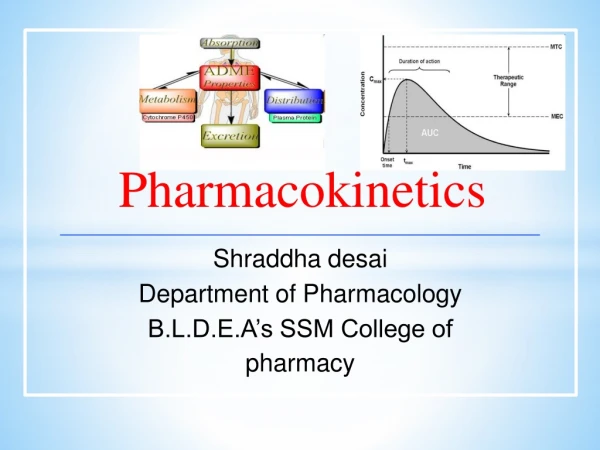
Absorption
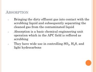
Absorption. Bringing the dirty effluent gas into contact with the scrubbing liquid and subsequently separating the cleaned gas from the contaminated liquid Absorption is a basic chemical enginnering unit operation which in the APC field is reffered as scrubbing

Absorption
E N D
Presentation Transcript
Absorption • Bringing the dirty effluent gas into contact with the scrubbing liquid and subsequently separating the cleaned gas from the contaminated liquid • Absorption is a basic chemical enginnering unit operation which in the APC field is reffered as scrubbing • They have wide use in controlling SO2, H2S, and light hydrocarbons
Absorption _Wet scrubbers can be categorized into 3 groups: • Packed-bed counterflow scrubbers • Cross-flow scrubbers • Bubble plate and tray scrubbers
Scrubber Types Packed Tower Spray tower Venturi Absorber
Concept of Absorption Gas absorption is the removal of one or more pollutants from a contaminated gas stream by allowing the gas to come into intimate contact with a liquid that enables the pollutatants to become dissolved by the liquid. The principal factor dictating performance is the solubility of the pollutants in the absorbing liquid. The rate of transfer in the liquid is dictated by the diffusion processes occurring on each side of the gas liquid interface.
Liquid Waste Pollutants removed from the gas stream transferred into liquid phase whose disposal is another issue to deal with. Therefore scrubber needs other units such as storage vessels, additives to treat the scrubbing liquid according to required discharge standards.
Absorption • Absorption units must provide large surface area of liquid-gas interface • Therefore the units are designed to provide large liquid surface area with a minimum of gas pressure drop
Packing Material and Shapes • Packing material (must be inert) is designed to increase the liquid-film surface • Many geometric shapes are available : Raschig ring, pall ring, berl saddle, tellerete etc.
Absorption Theory • Physically, the absorption of a pollutant gas from a moving gas stream into an appropriate liquid stream is quite complex • Basically the transfer process into each fluid stream is accomplished by 2 mechanisms: • The pollutant species is transferred from the bulk of the gas stream toward the gas-liquid interface by turbulent eddy motions • Very close to the interface laminant flow is valid and transfer is accomplished by molecular diffusion • On the liquid side of the interface process is reversed
Absorption Theory • On the basis of Fick's Law, the diffusion of one gas (A) through a second stagnant gas B, NA, the molar rate of transfer of A per unit cross-sectional area is given by; • NA = -DAB (dcA/dz)/(1-(cA/c) DAB: molecula diffusion coef. (m2/t) cA: molar concentration of species A (mol/L) c: molar concentration of the gas mixture (mol/L) z: the direction of mass transfer (m) • DAB tables are available for a number of binary gas mixtures
Absorption Theory • Mass transfer rate per unit area for molecular diffusion of A through a second liquid is given by: • NA = -DL/z (cA2-cA1) DL: liquid phase molecular diffusion coef. (m2/t) cA2-cA1: concentration difference of A over the distance z • Typical values of DL for binary mixtures are tabulated in the literature.
The Equilibrium Distribution Curve • Before entering into details of mass transfer, let's summarize the method of presenting equilibrium data for a pollutant A distributed between liquid and gas phase P=c Inject solute A Inert Liquid Solvent Inert carrier gas Mole fraction in gas, yA Exp. Equilib. Distribution curve Mole fraction in lqiuid, xA
The Equilibrium Distribution Curve • After sufficient time, no further change in the concentration of A in two phases. These concentration can be measured and converted into mole fraction xA in the liquid phase and yA in the gas phase P=c Inject solute A Inert Liquid Solvent Inert carrier gas Mole fraction in gas, yA Exp. Equilib. Distribution curve Mole fraction in lqiuid, xA
Mass transfer coefficients based on Interfacial Concentrations • When mass transfer occurs in moving liquid and gaseous streams, it is difficult to evaluate the separate effects of molecular and turbulent diffusion • An alternative to this is to express NA for each phase in terms of mass transfer coefficient k and a driving force based on the bulk and interfacial concentrations for that phase
Mass transfer coefficients based on Interfacial Concentrations • For the liquid phase: • NA = kL(cAi-cAL) = kx(xAi-xAL) • kL(is the liquid mass transfer coeff. Based on concentration, in length per unit of time, cAiis the concentration of A in the liquid phase at the interface, cALis the concentration of A in the bulk of the phase, in moles per unit volume. • kx is the liquid mass transfer coefficient based on mole fractions, in moles per units of time and length squared, xA is the mole fraction of A in the liquid interface, and xAL is the mole fraction of A in the bulk of the liquid phase
Mass transfer coefficients based on Interfacial Concentrations • For the gas phase: • NA = kG(pAG-cAi) = ky(yAG-yAi) • kGis the gas phase mass transfer coeff. based on partial pressures, in moles/length2 time, pAGis the partial pressure of A in the bulk of gas phase pAi is the partial pressure of A in the gas interface • ky is the gas phase mass transfer coefficient based on mole fractions, in moles per units of time and length squared, yAG is the mole fraction of A in the bulk of the gas phase, and yAi is the mole fraction of A in the gas phase interface
Mass transfer coefficients based on Interfacial Concentrations • However this approach to determining NA is not practical since kx and ky are difficult to obtain and no way to measure the values of yAi and xAi experimentally since any attempt to do it will perturb the equilibrium between the two streams
Overall Mass Transfer Coefficients • When mass transfer rates are reasonably low, NA can be expressed as: • NA = KG(pAG-pA*) = Ky(yAG-yA*) • KG and Ky are local overall mass transfer coefficients • pA* : equilibrium partial pressure of solute A in a gas phase which is in contact with a liquid having the composition of cAL of the main body of the absorption liquid • yA*: defined similarly in terms of a liquid with mole fraction xAL of the bulk liquid
Overall Mass Transfer Coefficients Point P represents the state of the bulk phase of the 2 fluid streams, yAG and xAL. The point M represents the state (yAi and xAi) associated with equilibrium at the interface The distance between P and C is a measure of the driving force. slope=m'
Overall Mass Transfer Coefficients • NA = KG(pAG-pA*) = Ky(yAG-yA*) This equation is usually restricted the resistance to mass transfer is primarily in the gas phase, which characterizes the majority of absorption problems in air pollution work • The solubility of the polutant gas normally determines the liquid that is chosen • The major physical problem is getting the pollutant to diffuse through the gas phase to the interface, consequently gas phase controls the process. • If the liquid phase controls: • NA = KL(cA*-cAL) = Kx(xA*-xAL)
Overall Mass Transfer Coefficients • It is important to note that the quantities pA*,yA*,cA*,xA* do not represent any actual condition in the absorption process but are related in each case to a real concentration in one of the bulk fluids through the equilibrium data for the two-phase system. From the geometry of the previous figure: • yAG-yA*= yAG-yAi+(yAi-yA*) • yAi-yA*=m'(xAi-xAL) • yAG-yA*= yAG-yAi+m'(xAi-xAL) • 1/Ky=1/ky+m'/kx
Mass Balances and the Operating Line for Packed Towers Gm molar total gas flow rate (carrier gas + pollutant) Gc molar inert carrier gas flow rate Lm molar total solvent flow rate (solvent + absorbed pollutant) Ls molar solvent flow rate x is the liquid mole fraction of pollutant, y is the gas phase mole fraction of the pollutants, X is the liquid phase mole ratio and Y is the gas phase mole ratio Lm,2 Ls x2 X2 Gm,2 Gc y2 Y2 T = const P = const Cross-sectional area, A dz Gm,1 Gc y1 Y1 Lm,1 Ls x1 X1
Mass Balances and the Operating Line for Packed Towers • Mole fraction and mole ratio: • X = x/(1-x) Y = y/(1-y) • Subscript m denotes that rates are in the units of mole basis • The conservation of mass principle applied to the pollutant species in terms of total mass flow rates at top and bottom yields: Gm,1y1+ Lm,2x2 = Gm,2y2+ Lm,1x1 • or Gm,1y1 -Gm,2y2 = Lm,1x1 -Lm,2x2
Mass Balances and the Operating Line for Packed Towers • In Gm,1y1 -Gm,2y2 = Lm,1x1 -Lm,2x2 total gas and liquid flow rates are not equal at the top and the bottom of the column, therefore we cannot further simplify this equation. • When we write the equation in terms of the carrier gas and liquid solvent rates then: • GC,m(Y2-Y1) = LS,m(X2-X1) • These two equations above gives a straight line on Y-X coordinates with a slope of Lsm/GCm and called operating lines.
The operating line lies above the equilibrium line for absorption • For a stripping (removal of gas from liquid stream) the operating line must lie below the equilibrium line in order for the drving force to act from the liquid phase toward the gas phase Dirty air Clean air Clean water Dirty water
The Minimum and Design Liquid- Gas Ratio • At the bottom and top of the absorber, parameters Gm,1, Gc, y1, Gm2, y2, and x2 are known. • We need to determine Ls, and x1 • So we have one equation with 2 unknowns... • However selection of one of these values, obviously fixes the other. • How to select a value?
The Minimum and Design Liquid- Gas Ratio The minimum rate is highly undesirable. At this point driving force is almost 0. Hence it would take an infinetely tall absorber to accomplish the desired separation As a general operating principle an absorber is typically designed to operate at liquid rates which are 30 to 70 % greater than minimum rate.
Tower Diameter and Pressure Drop per Unit Tower Height • For a given packing and liquid flow rate in an absorption tower variation in the gas velocity has a significant effect on the pressure drop • As the gas velocity is increased, the liquid tends to be retarded in its downward flow, giving rise to term liquid holdup (LH) • A LH increases, the free cross-sectional area for gas flow decreases and pressure drop per unit height increases.
Problems with High Gas Velocity • Channeling: the gas or liquid flow is much greater at some points than at others • Loading: the liquid flow is reduced due to the increased gas flow; liquid is held in the void space between packing • •Flooding: the liquid stops flowing altogether and collects in the top of the column due to very high gas flow • TO AVOID this condition experience dictates operating at gas velocities which are 40 to 70 % of those which causing flooding
Flood Point • The relationship between DP/Z and other important tower variables-liquid and gas rates, liquid and gas stream densities and viscosities, and type of packing has been extensively studied on an experimental basis. • A widely accepted correlation among these parameters can be seen in below figure • Where G' and L': superficial gas and liquid mass flow rate defined as actual flow rates divided by the empty cross-sectional area of the tower.
L’/G’√(rG/rL-rG) L’: liquid mass flux (lb/s-ft2) G’:gasmassflux (lb/s-ft2) F:packing factor (ft2/ft3) mL:liquidviscosity, cp gc: proportıonalityconstant, 32.17 ft-lb/s2-lbf rL:liquiddensity, lb/ft3 rG:gasdensity, lb/ft3 In Cooper and Alley’s book, Figure 13.6 can be used. Note that in Figure 13.6 Gx and Gy are liquid and gas flux (lg/s-ft2), respectively. In our notation G’ and L’ correspond to Gx and Gy
PackingFactor F • The top line in the figure represents the general flooding condition for many packings. The flooding condition however has been found to vary as a function of the packing factor F (dimensionless packing factor tabulated below) • Recent studies showed that when F is in the range of 10 to 60, the pressure drop can be expressed by: DPflood = 0.115F0.7
Determining Tower Diameter • First abscissa value is calculated (L'/G')(pG/(pL-pG))0.5 • Where this value intercepts the flooding line on Figure A, move horizontally to the left and read the value of the ordinate: (G')2F(mL)0.1/gc(pL-pG)pG • Calculate the G’ and take 30 to 70% of it to prevent flooding • Tower crossectional area: A = G/G‘ • Evaluate the tower diameter
Determining Expected Pressure Drop per Unit Height of Tower • First calculate actual G’ and L’ and then calculate the abscissa and the ordinate for use in Figure 13.6 • From those values the intersection on the figure defines the pressure drop per foot of packed height Another emprical correlation found in the litrature for the DP in packing when operating below the load point is DP/Z = 10-8m[10nL’/rL](G’2/rG) m and n are packing constants see Table 6.2
Determining Tower Diameter and Expected Pressure Drop per Unit Height of Tower
Example A packedtower is to be designedtoremove 95% of theammoniafrom a gaseousmixture of 8 percentammoniaand 92% air, byvolume. Theflow rate of thegasmixtureenteringthetower at 68 F and 1 atm is 80 lb-moles/hr. Watercontaining no ammonia is to be thesolvent, and 1-in. Ceramicraschigringswill be used as thepacking. Thetower is tooperated at 60% of thefloodpointandtheliquidwater rate is to be 30% greaterthanthe minimum rate. Determine • 1. Thegas-phaseflowrates, in lb-moles/hr, forthesoluteandcarriergas • 2. Themoleratios of thegasandliquidphases at inlet andoutletandtherequiredwater rate in lbmoles/hr. • 3.Thegasandliquidrates (lb/hr) forcarriergas, solutegas, total gas, liquidsolvent, solute in liquid, and total liquid • 4. Thetowerareaanddiameter • 5. Thepressuredropbased on thetwomethodsgiven in thelecturenotes.
Example Removal efficiency: 95% Effluent Stream Composition: 8% ammonia and 92% air Gas T and P: 68F and 1 atm Flowrate: 80 lb-moles/hr Liquid phase: Containing no ammonia
Example Determine composition of the liquid at the exit (X1) (Inlet liquid concentration since pure water is used is x2=X2=0) Use equilibrium data for ammonia-air-water mixtures which are given below for 68 F and 14,7 psia. : In order to determine composition of liquid at the exit, we need to calculate the minimum solvent flow rate first. By plotting X vrs Y at the equilibrium, we can evaluate the minimum solvent and then operating solvent rate. In Cooper and Alley’s book, use Table B4 in the Appendix.
Example 0,90 Y2=0.00435 0.092 Since the liquid rate is to be 30% greater than the miniumu rate (Lm,S)/Gm,C)design = 1,30(0.90) = 1.17 mole/mole Lm,S = Gm,C*1,17 = 1.17*73.6 = 86.1 lb moles/hr
0,1 Y1=0.087 0,08 y, moles solute per mole 0,06 carrier gas (Lm,S/Gm,C)=1.17 0,04 0,02 X2,Y2 0.00435 0 0,02 0,04 0,06 0,08 0,1 X, moles solute per mole solvent Example 0,90 X1: 0.0707 Now, X1 can now be found. Graphically by drawing operating line with a slope of 1.17 with starting point of (0, 0.00435) and the point crosses Y1=0.087 can be read. OR From Lms/Gm,C = Y2-Y1/(X2-X1)=0.00435-0.087/(0-X1) = 1.17 X1 = 0.0707 lm mole A/lm mole water or x1 = 0.066 lb mole A /lb moles solution
FlowRates Lm,2 Ls x2 X2 The gas and liquid rates: GC = 73.6*29 = 2134 lb/hr GA,1 = 6.4*17 = 109 lb/hr GA,2 = 0.32*(17) = 5.4 lb/hr LS = 86.1*18=1550 lb/hr LA,1 = DGA= 109*0.95=104 lb/hr Therefore: G1 = 2134 +109=2243 lb/hr bottom L1 = 1550 +104 = 1654 lb/hr G2 = 21345+5=2139 lb/hr top L2=1550 + 0 = 1550 lb/hr top Gm,2 Gc y2 Y2 T = const P = const Cross-sectional area, A dz Lm,1 Ls x1 X1 Gm,1 Gc y1 Y1
TowerArea To determine the tower area, we need to use Figure flooding correlation plot. Therefore we need to calculate gas and liquid phase densities at the top and bottom of the tower. Since the ammonia content is very low in liquid phase, use the density of pure water, 62.3 lb/ft3 as the solution density through the tower. For the gas phase assume ideal gas behavior: r= P/RT = MwP/RT At the top: Mw= SyiMi = 0.00435*17 + 0.9957*29 = 28.95 r= 28.95*14.7/(10.73*528) = 0.075 lb/ft3 At the bottom Mw= 0.08*17 + 0.92*29 = 28.04 r= 28.04*14.7/(10.73*528) = 0.0728 lb/ft3 Now calculate the abscissa of Flooding Figure
PressureDrop Pressure drop can be determined from the flooding figure or from an emprical equation