Models With Two or More Quantitative Variables
460 likes | 504 Views
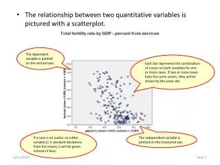
Learn about types of regression models with multiple quantitative variables, including models with interaction effects. Explore how the relationship between variables varies based on interactions, and run regressions to analyze these effects.

Models With Two or More Quantitative Variables
E N D
Presentation Transcript
Models With Two or More Quantitative Variables EPI809/Spring 2008
Types of Regression Models EPI809/Spring 2008
First-Order Model With 2 Independent Variables • Relationship Between 1 Dependent & 2 Independent Variables Is a Linear Function • Assumes No Interaction Between X1 & X2 • Effect of X1 on E(Y) Is the Same Regardless of X2 Values EPI809/Spring 2008
First-Order Model With 2 Independent Variables • Relationship Between 1 Dependent & 2 Independent Variables Is a Linear Function • Assumes No Interaction Between X1 & X2 • Effect of X1 on E(Y) Is the Same Regardless of X2 Values • Model EPI809/Spring 2008
No Interaction EPI809/Spring 2008
No Interaction E(Y) E(Y) = 1 + 2X1 + 3X2 12 8 4 0 X1 0 0.5 1 1.5 EPI809/Spring 2008
No Interaction E(Y) E(Y) = 1 + 2X1 + 3X2 12 8 4 E(Y) = 1 + 2X1 + 3(0) = 1 + 2X1 0 X1 0 0.5 1 1.5 EPI809/Spring 2008
No Interaction E(Y) E(Y) = 1 + 2X1 + 3X2 12 8 E(Y) = 1 + 2X1 + 3(1) = 4 + 2X1 4 E(Y) = 1 + 2X1 + 3(0) = 1 + 2X1 0 X1 0 0.5 1 1.5 EPI809/Spring 2008
No Interaction E(Y) E(Y) = 1 + 2X1 + 3X2 12 E(Y) = 1 + 2X1 + 3(2) = 7 + 2X1 8 E(Y) = 1 + 2X1 + 3(1) = 4 + 2X1 4 E(Y) = 1 + 2X1 + 3(0) = 1 + 2X1 0 X1 0 0.5 1 1.5 EPI809/Spring 2008
No Interaction E(Y) E(Y) = 1 + 2X1 + 3X2 E(Y) = 1 + 2X1 + 3(3) = 10 + 2X1 12 E(Y) = 1 + 2X1 + 3(2) = 7 + 2X1 8 E(Y) = 1 + 2X1 + 3(1) = 4 + 2X1 4 E(Y) = 1 + 2X1 + 3(0) = 1 + 2X1 0 X1 0 0.5 1 1.5 EPI809/Spring 2008
No Interaction E(Y) E(Y) = 1 + 2X1 + 3X2 E(Y) = 1 + 2X1 + 3(3) = 10 + 2X1 12 E(Y) = 1 + 2X1 + 3(2) = 7 + 2X1 8 E(Y) = 1 + 2X1 + 3(1) = 4 + 2X1 4 E(Y) = 1 + 2X1 + 3(0) = 1 + 2X1 0 X1 0 0.5 1 1.5 Effect (slope) of X1 on E(Y) does not depend on X2 value EPI809/Spring 2008
First-Order Model Worksheet Run regression with Y, X1, X2 EPI809/Spring 2008
Types of Regression Models EPI809/Spring 2008
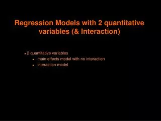
Interaction Model With 2 Independent Variables • Hypothesizes Interaction Between Pairs of X Variables • Response to One X Variable Varies at Different Levels of Another X Variable EPI809/Spring 2008
Interaction Model With 2 Independent Variables • Hypothesizes Interaction Between Pairs of X Variables • Response to One X Variable Varies at Different Levels of Another X Variable • Contains Two-Way Cross Product Terms EPI809/Spring 2008
Interaction Model With 2 Independent Variables 1. Hypothesizes Interaction Between Pairs of X Variables • Response to One X Variable Varies at Different Levels of Another X Variable 2. Contains Two-Way Cross Product Terms 3. Can Be Combined With Other Models • Example: Dummy-Variable Model EPI809/Spring 2008
Effect of Interaction EPI809/Spring 2008
Effect of Interaction 1. Given: EPI809/Spring 2008
Effect of Interaction 1. Given: 2. Without Interaction Term, Effect of X1 on Y Is Measured by 1 EPI809/Spring 2008
Effect of Interaction 1. Given: 2. Without Interaction Term, Effect of X1 on Y Is Measured by 1 3. With Interaction Term, Effect of X1 onY Is Measured by 1 + 3X2 • Effect changes As X2 changes EPI809/Spring 2008
Interaction Model Relationships EPI809/Spring 2008
Interaction Model Relationships E(Y) = 1 + 2X1 + 3X2 + 4X1X2 E(Y) 12 8 4 0 X1 0 0.5 1 1.5 EPI809/Spring 2008
Interaction Model Relationships E(Y) = 1 + 2X1 + 3X2 + 4X1X2 E(Y) 12 8 E(Y) = 1 + 2X1 + 3(0) + 4X1(0) = 1 + 2X1 4 0 X1 0 0.5 1 1.5 EPI809/Spring 2008
E(Y) 12 8 4 0 X1 0 0.5 1 1.5 Interaction Model Relationships E(Y) = 1 + 2X1 + 3X2 + 4X1X2 E(Y) = 1 + 2X1 + 3(1) + 4X1(1) = 4 + 6X1 E(Y) = 1 + 2X1 + 3(0) + 4X1(0) = 1 + 2X1 EPI809/Spring 2008
E(Y) 12 8 4 0 X1 0 0.5 1 1.5 Interaction Model Relationships E(Y) = 1 + 2X1 + 3X2 + 4X1X2 E(Y) = 1 + 2X1 + 3(1) + 4X1(1) = 4 + 6X1 E(Y) = 1 + 2X1 + 3(0) + 4X1(0) = 1 + 2X1 Effect (slope) of X1 on E(Y) does depend on X2 value EPI809/Spring 2008
Interaction Model Worksheet Multiply X1by X2 to get X1X2. Run regression with Y, X1, X2 , X1X2 EPI809/Spring 2008
Thinking challenge • Assume Y: Milk yield, X1: food intake and X2: weight • Assume the following model with interaction • Interpret the interaction ^ Y = 1 + 2X1 + 3X2 + 4X1X2 EPI809/Spring 2008
Types of Regression Models EPI809/Spring 2008
Second-Order Model With 2 Independent Variables • 1. Relationship Between 1 Dependent & 2 or More Independent Variables Is a Quadratic Function • 2. Useful 1St Model If Non-Linear Relationship Suspected EPI809/Spring 2008
Second-Order Model With 2 Independent Variables • 1. Relationship Between 1 Dependent & 2 or More Independent Variables Is a Quadratic Function • 2. Useful 1St Model If Non-Linear Relationship Suspected • 3. Model EPI809/Spring 2008
Second-Order Model Worksheet Multiply X1by X2 to get X1X2; then X12, X22. Run regression with Y, X1, X2 , X1X2, X12, X22. EPI809/Spring 2008
Models With One Qualitative Independent Variable EPI809/Spring 2008
Types of Regression Models EPI809/Spring 2008
Dummy-Variable Model 1. Involves Categorical X Variable With 2 Levels • e.g., Male-Female; College-No College 2. Variable Levels Coded 0 & 1 3. Number of Dummy Variables Is 1 Less Than Number of Levels of Variable • May Be Combined With Quantitative Variable (1st Order or 2nd Order Model) EPI809/Spring 2008
Dummy-Variable Model Worksheet X2 levels: 0 = Group 1; 1 = Group 2. Run regression with Y, X1, X2 EPI809/Spring 2008
Interpreting Dummy-Variable Model Equation EPI809/Spring 2008
Interpreting Dummy-Variable Model Equation Y X X Given: i 0 1 1 i 2 2 i Y Starting s alary of c ollege gra d' s X GPA 1 0 i f Male X 2 1 if Female EPI809/Spring 2008
Interpreting Dummy-Variable Model Equation Y X X Given: i 0 1 1 i 2 2 i Y Starting s alary of c ollege gra d' s X GPA 1 0 i f Male X 2 1 if Female Males ( X 0 ): 2 Y X X (0) i 0 1 1 i 2 0 1 1 i EPI809/Spring 2008
Interpreting Dummy-Variable Model Equation Y X X Given: i 0 1 1 i 2 2 i Y Starting s alary of c ollege gra d' s X GPA 1 0 i f Male X 2 1 if Female Same slopes Males ( X 0 ): 2 Y X X (0) i 0 1 1 i 2 0 1 1 i Females ( X 1 ): 2 Y X ( ) X (1) i 0 1 1 i 2 1 1 i 0 2 EPI809/Spring 2008
Dummy-Variable Model Relationships Y ^ Same Slopes 1 Females ^ ^ 0 + 2 ^ 0 Males 0 X1 0 EPI809/Spring 2008
Dummy-Variable Model Example EPI809/Spring 2008
Dummy-Variable Model Example Y 3 5 X 7 X Computer O utput: i 1 i 2 i 0 i f Male X 2 1 if Female EPI809/Spring 2008
Dummy-Variable Model Example Y 3 5 X 7 X Computer O utput: i 1 i 2 i 0 i f Male X 2 1 if Female Males ( X 0 ): 2 Y 3 5 X 7 3 5 X (0) i 1 i 1 i EPI809/Spring 2008
Dummy-Variable Model Example Y 3 5 X 7 X Computer O utput: i 1 i 2 i 0 i f Male X 2 1 if Female Same slopes Males ( X 0 ): 2 Y 3 5 X 7 3 5 X (0) i 1 i 1 i Females (X 1 ): 2 Y 3 5 X 7 (1) (3 + 7) 5 X i 1 i 1 i EPI809/Spring 2008
Sample SAS codes for fitting linear regressions with interactions and higher order terms PROC GLM data=complex; Class gender; model salary = gpa gendergpa*gender; RUN; EPI809/Spring 2008
Conclusion • Explained the Linear Multiple Regression Model • Tested Overall Significance • Described Various Types of Models • Evaluated Portions of a Regression Model • Interpreted Linear Multiple Regression Computer Output • Described Stepwise Regression • Explained Residual Analysis • Described Regression Pitfalls EPI809/Spring 2008