Download
1 / 85
860 likes | 1.02k Views
Basic frame of Genetic algorithm. Initialise a population Evaluate a population While (termination condition not met) do Select sub-population based on fitness Produce offspring of the population using crossover Mutate offspring stochastically. Evolution Runs Until:.

E N D
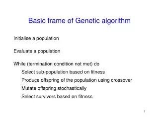
Basic frame of Genetic algorithm Initialise a population Evaluate a population While (termination condition not met) do Select sub-population based on fitness Produce offspring of the population using crossover Mutate offspring stochastically
Evolution Runs Until: A perfect individual appears (if you know what the goal is), Or: improvement appears to be stalled, Or: you give up (your computing budget is exhausted).
Simple GA Simulation Optimisation problem maximise the function f(x)=x2 x: integer between 0 and 31 objective function as the fitness function code using binary representation 110112 = 1910 1*24+0*23+0*22+1*21+1*20 0 is then 00000 31 is then 11111
Simple GA Simulation: Initial Population Lets assume that we want to create a initial population of 4 random flip coin 20 times (4 population size * string of 5) String Initial No. Population 1 01101 2 11000 3 01000 4 10011
Simple GA Simulation: Fitness Function String Initial f(x) Prob. = fi/Sum No. Population 1 01101 169 0.14 2 11000 576 0.49 3 01000 64 0.06 4 10011 361 0.31 Sum 1170 Average 293 Max 576
Simple GA Simulation: Roulette Wheel String Initial f(x) Prob Roulette. No. Population Wheel 1 01101 169 0.14 1 2 11000 576 0.49 2 3 01000 64 0.06 0 4 10011 361 0.31 1 Sum 1170 Average 293 Max 576
Simple GA Simulation: Mating Pool String Initial f(x) Prob Roulette. Mating No. Population Wheel Pool 1 01101 169 0.14 1 01101 2 11000 576 0.49 2 11000 3 01000 64 0.06 0 11000 4 10011 361 0.31 1 10011 Sum 1170 Average 293 Max 576
Simple GA Simulation: Mate String Initial f(x) Prob Roulette. Mating Mate No. Population Wheel Pool 1 01101 169 0.14 1 01101 2 2 11000 576 0.49 2 11000 1 3 01000 64 0.06 0 11000 4 4 10011 361 0.31 1 10011 3 Sum 1170 Average 293 Mate is Randomly selected Max 576
Simple GA Simulation: Crossover String Initial f(x) Prob R. Mating Mate Crossover No. Population W Pool 1 01101 169 0.14 1 01101 2 4 2 11000 576 0.49 2 11000 1 4 3 01000 64 0.06 0 11000 4 2 4 10011 361 0.31 1 10011 3 2 Sum 1170 Average 293 Crossover is Randomly selected Max 576
Simple GA Simulation: New Population String Initial f(x) Prob R. Mating Mate Cross New No. Population W Pool over Pop. 1 01101 169 0.14 1 01101 2 4 01100 2 11000 576 0.49 2 11000 1 4 11001 3 01000 64 0.06 0 11000 4 2 11011 4 10011 361 0.31 1 10011 3 2 10000 Sum 1170 Average 293 Max 576
Simple GA Simulation: Mutation String Initial f(x) Prob R. Mating Mate Cross New No. Population W Pool over Pop. 1 01101 169 0.14 1 01101 2 4 01100 2 11000 576 0.49 2 11000 1 4 11001 3 01000 64 0.06 0 11000 4 2 11011 4 10011 361 0.31 1 10011 3 2 10000 Sum 1170 Average 293 Max 576
Simple GA Simulation: Mutation String Initial f(x) Prob R. Mating Mate Cross New No. Population W Pool over Pop. 1 01101 169 0.14 1 01101 2 4 01100 2 11000 576 0.49 2 11000 1 4 10001 3 01000 64 0.06 0 11000 4 2 11011 4 10011 361 0.31 1 10011 3 2 10000 Sum 1170 Average 293 Max 576
Simple GA Simulation: Evaluation New Population String Initial f(x) Prob R. Mating Mate C New f(x) No. Population W Pool o Pop. 1 01101 169 0.14 1 01101 2 4 01100 144 2 11000 576 0.49 2 11000 1 4 10001 289 3 01000 64 0.06 0 11000 4 2 11011 729 4 10011 361 0.31 1 10011 3 2 10000 256 Sum 1170 1418 Average 293 354 Max 576 729
Problem & Representations Chromosomes represent problems' solutions as genotypes They should be amenable to: Creation (spontaneous generation) Evaluation (fitness) via development of phenotypes Modification (mutation) Crossover (recombination)
How GAs Represent Problems' Solutions: Genotypes Bit strings -- this is the most common method Strings on small alphabets (e.g., C, G, A, T) Permutations (Queens, Salesmen) Trees (Lisp programs). Genotypes must allow for: creation, modification, and crossover.
Binary-Encoding for Genetic Algorithms The original formulation of genetic algorithms relied on a binary encoding of solutions, i.e., the chromosomes consist of a string of 0’s and 1’s. No restriction on the phenotype so long as a good method for encoding/decoding exists. Other methods of encoding will come later.
Genetic Binary Encoding/Decoding of Integers Initially, single parameters Integer parameters: p is an integer parameter to be encoded. 3 distinct cases to consider: Case 1 p takes values from {0, 1, 2, …..2^N-1} for some N. In this case, p can be encoded by its equivalent binary representation.
Genetic Binary Encoding/Decoding of Integers Case 2 p takes values from {M, M+1, …., M+2^N-1} for some M, N. In this case (p-M) can be encoded directly by its equivalent binary representation. Case 3 p takes values from {0, 1, .., L-1} for some L such that there exist no N for which L=2^N. There are two possibilities. Clipping and Scaling
Clipping Take N = log(L)+1 and encode all parameter values 0<= p <= L-2 by their equivalent binary representation, letting all other n-bit strings serve as encodings of p = L-1. Example: p from {0,1,2,3,4,5}, i.e., L=6. Then N=log(6)+1= 3 p 0 1 2 3 4 5 5 5 Code 000 001 010 011 100 101 110 111 Advantages: Easy to implement Disadvantages: Strong representational bias. All parameter values between 0 and L-2 have a single encoding, but the single value L-1 has 2^N-L+1 encodings
Scaling Take N=log(L)+1 and encode p by the binary representation of the integer e such that p = e(L-1)/(2^N-1) Example: p from {0,1,2,3,4,5} i.e. L=6, N=log(6)+1=3. p 0 0 1 2 2 3 4 5 Code 000 001 010 011 100 101 110 111 Advantages: Easy to implement. Smaller representational bias than clipping (at most double representations) Disadvantages: Small representational bias. More computation than clipping.
Gray Coding Desired: points close to each other in representation space also close to each other in problem space This is not the case when binary numbers represent floating point values Binary gray code 000 000 001 001 010 011 011 010 100 110 101 111 110 101 111 100
Gray Coding m is number of bits in representation Binary number b = (b1; b2; ; bm) Gray code number g = (g1; g2; ; gm)
Gray Coding PROCEDURE Binary-To-Gray g1=b1 for k=2 to m do gk=b k-1 XOR bk endfor
Gray Coding PROCEDURE Gray-To-Binary value = g1 b1 = value for k = 2 to m do if gk = 1 then value = NOT value end if bk =value end for
Binary Encoding and Decoding of Real-valued parameters Can be encoded as: fixed-point numbers integers using scaling and quantisation If p ranges over [min,max] encode p using N bits by using the binary representation of the integer part of (2^N-1)(p-min)/(max - min)
Multiple parameters Vectors of parameters are encoded on multi-gene chromosomes by combining the encodings of each individual parameter. Let e_i =[b_i0,….b_iN] be the encoding of the ith of M parameters. There are two ways of combining the e_i’s into a chromosome. Concatenating: Individual encodings simply follow one another in some predefined order e.g. [b_10,…b_1N,..,b_M0,…b_MN] Interleaving: the bits of each individual encoding are interleaved e.g. [b_10,…,b_M0,b_11,…,b_MN] The order of parameters in the vector (i.e. genes in the chromosome) is important, especially for concatenated encodings.
Initialization Initialise a population Evaluate a population While (termination condition not met) do Select sub-population based on fitness Produce offspring of the population using crossover Mutate offspring stochastically
Initialization init( ) { for( i = 0; i < POP_SIZE; i++ ) for( j = 0; j < N; j++ ) p[i][j] = random_int( 2 ); }
GA Main Program Initialise a population Evaluate a population While (termination condition not met) do Select sub-population based on fitness Produce offspring of the population using crossover Mutate offspring stochastically
GA Main Program for( trial = 0; trial < LOOPS; trial++ ) { selection( ) crossover( ) mutation( ) for( who = 0; who < POP_SIZE; who++ ) fitness[who] = fv(who); }
Selection Initialise a population Evaluate a population While (termination condition not met) do Select sub-population based on fitness Produce offspring of the population using crossover Mutate offspring stochastically
Selection Selects individuals for reproduction • randomly with a probability depending on the relative fitness of the individuals so that the best ones are more often chosen for reproduction rather than poor ones • Proportionate-based selection picks out individuals based upon their fitness values relative to the fitness of the other individuals in the population • Ordinal-based selection selects individuals based upon their rank within the population; independent of the fitness distribution
Roulette Wheel Selection Here is a common technique: let F = j=1 to popsizefitnessj Select individual k with probability fitnessk/F
Roulette Wheel Selection assigns to each solution a sector of a roulette wheel whose size is proportional to the appropriate fitness measure chooses a random position on the wheel (spin the wheel) c Fitness a:1 b:3 c:5 d:3 e:2 f:2 g:8 b d a e g f
Roulette Wheel Realization For each chromosome evaluate the fitness and the cumulative fitness For N times create a random number Select the chromosome where its cumulative fitness is the first value greater than the generated random number Individual Chromosome Fitness Cumulative x1 101100 20 20 x2 111000 7 27 x3 001110 6 33 x4 101010 10 43 x5 100011 12 55 x6 011011 9 64
Roulette Wheel Example Individual Chromosome Fitness Cumulative Random Individual x1 101100 20 20 42.8 x2 111000 7 27 x3 001110 6 33 x4 101010 10 43 x5 100011 12 55 x6 011011 9 64
Roulette Wheel Example Individual Chromosome Fitness Cumulative Random Individual x1 101100 20 20 42.8 x4 x2 111000 7 27 x3 001110 6 33 x4 101010 10 43 x5 100011 12 55 x6 011011 9 64
Roulette Wheel Example Individual Chromosome Fitness Cumulative Random Individual x1 101100 20 20 42.8 x4 x2 111000 7 27 19.78 x3 001110 6 33 x4 101010 10 43 x5 100011 12 55 x6 011011 9 64
Roulette Wheel Example Individual Chromosome Fitness Cumulative Random Individual x1 101100 20 20 42.8 x4 x2 111000 7 27 19.78 x1 x3 001110 6 33 x4 101010 10 43 x5 100011 12 55 x6 011011 9 64
Roulette Wheel Example Individual Chromosome Fitness Cumulative Random Individual x1 101100 20 20 42.8 x4 x2 111000 7 27 19.78 x1 x3 001110 6 33 42.73 ? x4 101010 10 43 58.44 ? x5 100011 12 55 27.31 ? x6 011011 9 64 28.31 ?
Roulette Wheel Example Individual Chromosome Fitness Cumulative Random Individual x1 101100 20 20 42.8 x4 x2 111000 7 27 19.78 x1 x3 001110 6 33 42.73 x4 x4 101010 10 43 58.44 x6 x5 100011 12 55 27.31 x3 x6 011011 9 64 28.31 x3
Roulette Wheel Selection There are some problems here: fitnesses shouldn't be negative only useful for max problem probabilities should be “right” avoid skewing by super heros.
Parent Selection: Rank Here is another technique. Order the individuals by fitness rank Worst individual has rank 1. Best individual has rank POPSIZE Let F = 1 + 2 + 3 + + POP_SIZE Select individual k to be a parent with probability rankk/F Benefits of rank selection: the probabilities are all positive can be used for max and min problems the probability distribution is “even”
Parent Selection: Rank Power Yet another technique. Order the individuals by fitness rank Worst individual has rank 1. Best individual has rank POP_SIZE Let F = 1s + 2s + 3s + + POP_SIZEs Select individual k to be a parent with probability rankks/F benefits: the probabilities are all positive can be used for max and min problems the probabilities can be skewed to use more “elitist” selection
Tournament Selection Pick k members of the population at random select one of them in some manner that depends on fitness
Tournament Selection void tournament(int *winner) { int size = tournament_size, i, winfit; for( i = 0; i < size; i++ ) { int j = random_int( POP_SIZE );; if( j==0 || fitness[j] > winfit ) winfit = fitness[j],*winner = j; } }
Truncation selection Choose the best k individuals as the offspring There is no randomness If the population size is N, some researchers suggest k/N=0.3
Crossover Methods Initialise a population Evaluate a population While (termination condition not met) do Select sub-population based on fitness Produce offspring of the population using crossover Mutate offspring stochastically
Crossover Methods Crossover is a primary tool of a GA. (The other main tool is selection.) CROSS_RATE: determine if the chromosome attend the crossover Common techniques for bit string representations: One-point crossover: Parents exchange a random prefix Two-point crossover: Parents exchange a random substring Uniform crossover: Each child bit comes arbitrarily from either parent (We need more clever methods for permutations & trees.)
1-point Crossover Suppose we have 2 strings a and b, each consisting of 6 variables a1, a2, a3, a4, a5, a6 b1, b2, b3, b4, b5, b6 representing two solutions to a problem a crossover point is chosen at random and a new solution is produced by combining the pieces of the original solutions if crossover point was 2 a1, a2, b3, b4, b5, b6 b1, b2, a3, a4, a5, a6