Capacity Demand Curve for the Office of the Massachusetts Attorney General

1. Capacity Demand Curve for the Office of the Massachusetts Attorney General Feb. 27th , 2014 Prepared By: Randell Johnson Andrew Bachert Energy Exemplar MA AGO

2. Guiding Principles • Determine a peak price of capacity curve that will minimize the build costs, production cost (E&AS), and shortage costs (VOLL*Unserved Energy) to achieve on a target 1 day in 10 year LOLE reliability metric • Consider load risk impact during LOLE simulations • Assess price volatility of the capacity demand curve • Reconcile results with other regional markets • Review magnitude of incentives at peak price and rate of return on equity for investments MA AGO

3. Description of Optimization • PLEXOS optimization determines the minimum net present value (NPV) of the system in terms of investments, production cost, ancillary services cost, and shortage costs • Subject to constraints of: • Meeting demand • Feasible builds • Feasible production • 1 in 10 LOLE reliability standard • and others • Investments are additional production, demand response, or other equipment of the system to meet constraints and at lowest cost • Production cost is the short run marginal cost of the system to supply load subject to constraints • Ancillary services cost is the additional costs for meeting reserve provisions • Shortage Costs are costs when there is loss of load and these costs are a value of lost load (VOLL) multiplied by the unserved energy • Capacity payments help to minimize shortage costs Capacity Demand Curve has impact to least cost optimization MA AGO

4. Least Cost Optimization Objective: Minimize net present value of the sum of investment and production costs over time Cost $ Investment cost/ Capital cost C(x) • Chart shows the minimization of total cost of investments and of production cost • As more investments made production cost trends down however investment cost trends up Total Cost = C(x) + P(x) Production Cost P(x) Minimum cost plan x Investment x MA AGO

5. Cost Minimization with Capacity Curve Peak Price Cont. • Objective: • Minimize net present value of capital costs, production costs, ancillary costs, ancillary shortages, demand shortages • Minimize: • [Build Cost]+[Production Cost]+[Demand Shortage Cost]+[Ancillary Services Shortage Cost] • Subject to: • [Electric Production] + [Electric Shortage] = [Electric Demand] + [Electric Losses] • [Ancillary Service Provision] >= [Ancillary Services Requirements] • [Electric Production] and [Ancillary Services Provision] feasible • [Build]<=[Max Build] • [Production]<=[Production Max] • [Intergrality] i.e. whole blocks of capacity • others MA AGO

6. Illustrative Least Cost Optimization Due to time constraints method partially tested with one year optimization Investment Cost Production Cost Individual Unit Production Individual Unit Production Cost VOLL Unserved Energy Individual Unit Build Cost Amount Built This simplified illustration shows the essential elements of the PLEXOS mixed integer programming formulation for determination of a demand capacity curve that would achieve a target reliability level of LOLE at 1-in-10. PLEXOS also has many other variables and costs as part of the optimization such as capacity payments as well as other possible constraints = for all = year = interval = unit Y = Horizon MA AGO

7. Least Cost Optimization with Capacity Demand Curve Explanation of Terms • = Capital Cost • = Capacity Built by Type • = Individual Unit Production • = VOLL • = Unserved Energy • = MW Demand • = Max Capacity of individual Units • = Max Build Capacity by Type • = Target LOLE • Symbol means: for all • ∑ Symbol Means: sum up the individual items MA AGO

8. Features of Capacity Demand Curve MA AGO

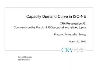
9. MA AGO Capacity Demand Curve Start of Downward Slope Peak Price NICR Crossing Point Kink Foot NICR LOLE: 1-in-10 MA AGO

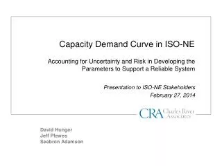
10. Comparison of Capacity Demand Curves NICR LOLE: 1-in-10 Initial Candidate Curve, NY Curve, PJM Curve coordinates estimated from MC materials: “Draft Recommendations for a Capacity Demand Curve in ISO-NE”, Slide 15, Jan 14, 2014 MA AGO

11. Calculated 1-in-10 LOLE 160 PLEXOS Simulations of High Level ISO-NE Control Area Model Results: NICR = 33,855 MW LOLE = 0.1 - Simulated load risk in calculating LOLE - Simulated multiple capacity levels MA AGO

12. Net CONE: many multiples of plant FOM Source: New Entrants Data from MC Feb 27 Net CONE presentation MA AGO

13. MA AGO Curve Reduces Price Volatility Compared to Initial Candidate Curve MA AGO

14. Net CONE Benchmarks • Net CONE Assumes a 13.8% Equity Rate of Return for the following technologies: • 4 x LM 6000: $20.60/kW-m • 2 x LMS 100: $17.85/kW-m • 2 x Frame CT: $ 8.95/kW-m • 2 x 1 Combined Cycle: $11.71/kw-m • This was done by solving the Net CONE value in $ / kW-month for each technology given a specific rate of return for equity of 13.8%. The financial models for these calculations are complex and include a number of different assumptions and properties. • The following analysis reviews the equity rate of returns for these same projects assuming different Net CONE assumptions. Source: MC Feb 27th Net CONE Presentation MA AGO

15. Net CONE Benchmarks (continued) First, we benchmarked each technology based on their Net CONE values and the 13.8% equity rate of return. Economic Life: 20 years Debt Leverage: 50% of Overnight Project Cost Debt Amortization: standard amortization over 10 years Debt Interest rate: 7.0% Tax Depreciation: MACRS 15 Year Depreciation for the LMS and CT and 20 Year for CC Corporate Tax Rate: 35% Inflation Rate: 2.25% Size and cost of plant as per the Feb 27, 2014 Presentation Source: MC Feb 27th Net CONE Presentation MA AGO

16. ROE for Peak Price MA AGO

17. Capacity Clearing Price of 1.6 x $11.71/kW-m • Assuming a capacity price of $18.73/kW-m for the new Capacity Resources, the Equity Rate of Return for these same hypothetical projects would be a follows: • 4 x LM 6000: 12.0% • 2 x LMS 100: 14.8% • 2 x Frame CT: 35.0% • 2 x 1 Combined Cycle: 25.3% • Again, the LM 6000 project would face a slight degradation of equity returns from 13.8% to 12.0%, but the other projects have a significantly improved results relative to their original position. These results also suggest that the returns are far in excess of market expectation at that capacity price for several technologies. MA AGO

18. Capacity Clearing Price of 2 x $11.71/kW-m • Finally, assuming a value 2 x $11.71 /kW-m, the Equity Rate of Return for these same hypothetical projects would increase as follows: • 2 x LM 6000: 16.5% • 2 x LMS 100: 19.9% • 2 x Frame CT: 45.3% • 2 x 1 Combined Cycle: 33.1% • In this case, all projects have a significantly improved results relative to their original net cone economics. These results also suggest that the returns are far in excess of market expectation at that capacity price for several technologies. MA AGO

19. ROE Comparison for Net CONE Multipliers of 1.6 and 2 With Net CONE of 11.71 and 2x Net CONE Multiplier Excess Equity Returns Possible MA AGO

20. Recommendations of Future Capacity Demand Curve • Consider a 20 year outlook for development of Capacity Demand Curve shape • Consider least cost constrained optimization of short run and long run marginal costs including minimization of the value of lost load • Run multiple scenarios of technologies, demands, fuel prices, and possibly others and allow the optimization to deactivate units if necessary for least cost system development • Use a stakeholder driven process for the above MA AGO