Standard Deviation
Standard Deviation. Lecture 18 Sec. 5.3.4 Mon, Feb 18, 2007. Variability. Our ability to estimate a parameter accurately depends on the variability of the population. What do we mean by variability in the population? How do we measure it?. Deviations from the Mean.

Standard Deviation
E N D
Presentation Transcript
Standard Deviation Lecture 18 Sec. 5.3.4 Mon, Feb 18, 2007
Variability • Our ability to estimate a parameter accurately depends on the variability of the population. • What do we mean by variability in the population? • How do we measure it?
Deviations from the Mean • Each unit of a sample or population deviates from the mean by a certain amount. • Define the deviation of x to be (x –x). 1 2 3 4 6 7 8 9 10 5
Deviations from the Mean • Each unit of a sample or population deviates from the mean by a certain amount. • Define the deviation of x to be (x –x). 1 2 3 4 6 7 8 9 10 5 x = 6
Deviations from the Mean • Each unit of a sample or population deviates from the mean by a certain amount. deviation = –5 1 2 3 4 6 7 8 9 10 5 x = 4
Deviations from the Mean • Each unit of a sample or population deviates from the mean by a certain amount. dev = –2 1 2 3 4 6 7 8 9 10 5 x = 4
Deviations from the Mean • Each unit of a sample or population deviates from the mean by a certain amount. dev = +1 1 2 3 4 6 7 8 9 10 5 x = 4
Deviations from the Mean • Each unit of a sample or population deviates from the mean by a certain amount. dev = +2 1 2 3 4 6 7 8 9 10 5 x = 4
Deviations from the Mean • Each unit of a sample or population deviates from the mean by a certain amount. deviation = +4 1 2 3 4 6 7 8 9 10 5 x = 4
Deviations from the Mean • How do we obtain one number that is representative of the whole set of individual deviations? • Normally we use an average to summarize a set of numbers. • Why will the average not work in this case?
Sum of Squared Deviations • We will square them all first. That way, there will be no canceling. • So we compute the sum of thesquared deviations, called SSX.
Sum of Squared Deviations • Procedure • Find the average • Find the deviations from the average • Square the deviations • Add them up
Sum of Squared Deviations • SSX = sum of squared deviations • For example, if the sample is {1, 4, 7, 8, 10}, then SSX = (1 – 6)2 + (4 – 6)2 + (7 – 6)2 + (8 – 6)2 + (10 – 6)2 = (–5)2 + (–2)2 + (1)2 + (2)2 + (4)2 = 25 + 4 + 1 + 4 + 16 = 50.
The Population Variance • Variance of the population • The population variance is denoted by 2.
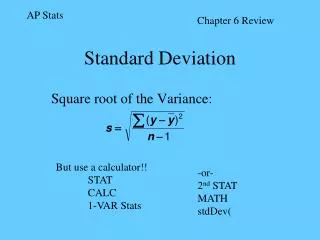
The Population Standard Deviation • The population standard deviation is the square root of the population variance.
The Sample Variance • Variance of a sample • The sample variance is denoted by s2.
The Sample Variance • Theory shows that if we divide by n – 1 instead of n, we get a better estimator of 2. • Therefore, we do it.
Example • In the example, SSX = 50. • Therefore, s2 = 50/4 = 12.5.
The Sample Standard Deviation • The sample standard deviation is the square root of the sample variance. • We will interpret this as being representative of deviations in the sample.
Example • In our example, we found that s2 = 12.5. • Therefore, s = 12.5 = 3.536. • How does that compare to the individual deviations?
Alternate Formula for the Standard Deviation • An alternate way to compute SSXis to compute • Then, as before
Example • Let the sample be {1, 4, 7, 8, 10}. • Then x = 30 and x2 = 1 + 16 + 49 + 64 + 100 = 230. • So SSX = 230 – (30)2/5 = 230 – 180 = 50, as before.
TI-83 – Standard Deviations • Follow the procedure for computing the mean. • The display shows Sx and x. • Sx is the sample standard deviation. • x is the population standard deviation. • Using the data of the previous example, we have • Sx = 3.535533906. • x = 3.16227766.
Interpreting the Standard Deviation • The standard deviation is directly comparable to actual deviations. • How does 3.536 compare to -5, -2, +1, +2, and +4?
Interpreting the Standard Deviation • Observations that deviate fromx by much more than s are unusually far from the mean. • Observations that deviate fromx by much less than s are unusually close to the mean.
Interpreting the Standard Deviation s s x – s x x + s
Interpreting the Standard Deviation A little closer than normal tox but not unusual x – s x x + s
Interpreting the Standard Deviation Unusually close tox x – s x x + s
Interpreting the Standard Deviation A little farther than normal fromx but not unusual x – 2s x – s x x + s x + 2s
Interpreting the Standard Deviation Unusually far fromx x – 2s x – s x x + s x + 2s