Download
1 / 53
530 likes | 549 Views
Explore camera projection, transformations, and geometric concepts in the world of computer vision. Learn about global parametric transformations, common linear and scaling operations, affine and projective transformations, and more.

E N D
Cameras and World Geometry How tall is this woman? How high is the camera? What is the camera rotation wrt. world? Which ball is closer? James Hays
Hays Things to remember • Pinhole camera model and camera (projection) matrix • Homogeneous coordinates allow projection as a matrix multiplication • Model approximates a camera • Lens distortion • Aperture
Parametric (global) transformations T Transformation T is a coordinate-changing machine: p’ = T(p) What does it mean that T is global? • T is the same for any point p T can be described by just a few numbers (parameters) For linear transformations, we can represent T as a matrix p’ = Tp p = (x,y) p’ = (x’,y’)
Common transformations Original Transformed Scaling Rotation Translation Perspective Affine Slide credit (next few slides): A. Efros and/or S. Seitz
Scaling • Scaling a coordinate means multiplying each of its components by a scalar • Uniform scaling means this scalar is the same for all components: 2
Scaling X 2,Y 0.5 • Non-uniform scaling: different scalars per component:
Scaling • Scaling operation: • Or, in matrix form: scaling matrix S
2-D Rotation (x’, y’) (x, y) y x’ = x cos() - y sin() y’ = x sin() + y cos() x
2-D Rotation This is easy to capture in matrix form: Even though sin(q) and cos(q) are nonlinear functions of q, • x’ is a linear combination of x and y • y’ is a linear combination of x and y What is the inverse transformation? • Rotation by –q • For rotation matrices R
Basic 2D transformations Scale Shear Rotate Translate Affine is any combination of translation, scale, rotation, and shear Affine
Affine Transformations Affine transformations are combinations of • Linear transformations, and • Translations Properties of affine transformations: • Lines map to lines • Parallel lines remain parallel • Ratios are preserved • Closed under composition or
2D image transformations (reference table) ‘Homography’ Szeliski 2.1
Projective Transformations Projective transformations are combos of • Affine transformations, and • Projective warps Properties of projective transformations: • Lines map to lines • Parallel lines do not necessarily remain parallel • Ratios are not preserved • Closed under composition • Models change of basis • Projective matrix is defined up to a scale (8 DOF)
Camera (projection) matrix Slide Credit: Savarese R,t jw X kw Ow iw x x: Image Coordinates: (u,v,1) K: Intrinsic Matrix (3x3) R: Rotation (3x3) t: Translation (3x1) X:World Coordinates: (X,Y,Z,1)
Homogeneous coordinates • Allows matrix form for 3D transformations • Take rotation • Now add translation
Homogeneous coordinates • Allows matrix form for 3D transformations • Take rotation • Now add translation with homogeneous coordinate
Camera (projection) matrix Slide Credit: Savarese R,t jw X kw Ow iw x x: Image Coordinates: (u,v,1) K: Intrinsic Matrix (3x3) R: Rotation (3x3) t: Translation (3x1) X:World Coordinates: (X,Y,Z,1) Extrinsic Matrix
Homogeneous coordinates • Projective • Point becomes a line To homogeneous From homogeneous Song Ho Ahn
How to calibrate the camera?(also called “camera resectioning”) Linear least-squares regression! James Hays
Least squares line fitting • Data: (x1, y1), …, (xn, yn) • Line equation: yi = mxi + b • Find (m, b) to minimize y=mx+b (xi, yi) Matlab: p = A \ y; (Closed form solution) Modified from S. Lazebnik
Example: solving for translation A1 B1 A2 B2 A3 B3 Given matched points in {A} and {B}, estimate the translation of the object
Example: solving for translation (tx, ty) A1 B1 A2 B2 A3 B3 Least squares setup
Example: discovering rot/trans/scale A1 B1 A2 B2 A3 B3 Given matched points in {A} and {B}, estimate the transformation matrix
World vs Camera coordinates James Hays
James Hays Calibrating the Camera Use an scene with known geometry • Correspond image points to 3d points • Get least squares solution (or non-linear solution) Known 3d world locations Known 2d image coords M Unknown Camera Parameters
How do we calibrate a camera? Known 2d image coords Known 3d world locations 880 214 43 203 270 197 886 347 745 302 943 128 476 590 419 214 317 335 783 521 235 427 665 429 655 362 427 333 412 415 746 351 434 415 525 234 716 308 602 187 312.747 309.140 30.086 305.796 311.649 30.356 307.694 312.358 30.418 310.149 307.186 29.298 311.937 310.105 29.216 311.202 307.572 30.682 307.106 306.876 28.660 309.317 312.490 30.230 307.435 310.151 29.318 308.253 306.300 28.881 306.650 309.301 28.905 308.069 306.831 29.189 309.671 308.834 29.029 308.255 309.955 29.267 307.546 308.613 28.963 311.036 309.206 28.913 307.518 308.175 29.069 309.950 311.262 29.990 312.160 310.772 29.080 311.988 312.709 30.514 James Hays
What is least squares doing? • Given 3D point evidence, find best M which minimizes error between estimate (p’) and known corresponding 2D points (p). . Error between M estimate and known projection point . . Z f Y . . v Camera center p’ under M u p = distance from image center
What is least squares doing? • Best M occurs when p’ = p, or when p’ – p = 0 • Form these equations from all point evidence • Solve for model via closed-form regression . Error between M estimate and known projection point . . Z f Y . . v Camera center p’ under M u p = distance from image center
Unknown Camera Parameters Known 2d image coords Known 3d locations First, work out where X,Y,Z projects to under candidate M. Two equations per 3D point correspondence James Hays
Unknown Camera Parameters Known 2d image coords Known 3d locations Next, rearrange into form where all M coefficients are individually stated in terms of X,Y,Z,u,v. -> Allows us to form lsq matrix.
Unknown Camera Parameters Known 2d image coords Known 3d locations Next, rearrange into form where all M coefficients are individually stated in terms of X,Y,Z,u,v. -> Allows us to form lsq matrix.
Unknown Camera Parameters • Finally, solve for m’s entries using linear least squares • Method 1 – Known 2d image coords Known 3d locations Ax=b form M = A\Y; M = [M;1]; M = reshape(M,[],3)'; James Hays
Unknown Camera Parameters • Or, solve for m’s entries using total linear least-squares. • Method 2 – Known 2d image coords Known 3d locations Ax=0 form [U, S, V] = svd(A); M = V(:,end); M = reshape(M,[],3)'; James Hays
How do we calibrate a camera? Known 2d image coords Known 3d world locations 880 214 43 203 270 197 886 347 745 302 943 128 476 590 419 214 317 335 783 521 235 427 665 429 655 362 427 333 412 415 746 351 434 415 525 234 716 308 602 187 312.747 309.140 30.086 305.796 311.649 30.356 307.694 312.358 30.418 310.149 307.186 29.298 311.937 310.105 29.216 311.202 307.572 30.682 307.106 306.876 28.660 309.317 312.490 30.230 307.435 310.151 29.318 308.253 306.300 28.881 306.650 309.301 28.905 308.069 306.831 29.189 309.671 308.834 29.029 308.255 309.955 29.267 307.546 308.613 28.963 311.036 309.206 28.913 307.518 308.175 29.069 309.950 311.262 29.990 312.160 310.772 29.080 311.988 312.709 30.514 James Hays
Known 2d image coords Known 3d world locations 1st point 880 214 43 203 270 197 886 347 745 302 943 128 476 590 419 214 335 … 312.747 309.140 30.086 305.796 311.649 30.356 307.694 312.358 30.418 310.149 307.186 29.298 311.937 310.105 29.216 311.202 307.572 30.682 307.106 306.876 28.660 309.317 312.490 30.230 307.435 310.151 29.318 ….. Projection error defined by two equations – one for u and one for v
Known 2d image coords Known 3d world locations 880 214 43 203 270 197 886 347 745 302 943 128 476 590 419 214 335 … 312.747 309.140 30.086 305.796 311.649 30.356 307.694 312.358 30.418 310.149 307.186 29.298 311.937 310.105 29.216 311.202 307.572 30.682 307.106 306.876 28.660 309.317 312.490 30.230 307.435 310.151 29.318 ….. 2nd point Projection error defined by two equations – one for u and one for v
How many points do I need to fit the model? 5 6 Degrees of freedom? • Think 3: • Rotation around x • Rotation around y • Rotation around z
How many points do I need to fit the model? 5 6 Degrees of freedom? M is 3x4, so 12 unknowns, but projective scale ambiguity – 11 deg. freedom. One equation per unknown -> 5 1/2 point correspondences determines a solution (e.g., either u or v). More than 5 1/2 point correspondences -> overdetermined, many solutions to M. Least squares is finding the solution that best satisfies the overdetermined system. Why use more than 6? Robustness to error in feature points.
Calibration with linear method • Advantages • Easy to formulate and solve • Provides initialization for non-linear methods • Disadvantages • Doesn’t directly give you camera parameters • Doesn’t model radial distortion • Can’t impose constraints, such as known focal length • Non-linear methods are preferred • Define error as difference between projected points and measured points • Minimize error using Newton’s method or other non-linear optimization James Hays
Can we factorize M back to K [R | T]? • Yes! • We can directly solve for the individual entries of K [R | T]. James Hays
an = nth column of A James Hays
Can we factorize M back to K [R | T]? • Yes! • We can also use RQ factorization (not QR) • R in RQ is not rotation matrix R; crossed names! • R (right diagonal) is K • Q (orthogonal basis) is R. • T, the last column of [R | T], is inv(K) * last column of M. • But you need to do a bit of post-processing to make sure that the matrices are valid. See http://ksimek.github.io/2012/08/14/decompose/ James Hays
Recovering the camera center This is not the camera center C. It is –RC, as the point is rotated before tx, ty, and tz are added t So we need -R-1 K-1 m4 to get C. m4 This is t × K So K-1 m4 is t Q is K × R. So we just need -Q-1 m4 Q James Hays
Estimate of camera center 1.5706 -0.1490 0.2598 -1.5282 0.9695 0.3802 -0.6821 1.2856 0.4078 0.4124 -1.0201 -0.0915 1.2095 0.2812 -0.1280 0.8819 -0.8481 0.5255 -0.9442 -1.1583 -0.3759 0.0415 1.3445 0.3240 -0.7975 0.3017 -0.0826 -0.4329 -1.4151 -0.2774 -1.1475 -0.0772 -0.2667 -0.5149 -1.1784 -0.1401 0.1993 -0.2854 -0.2114 -0.4320 0.2143 -0.1053 -0.7481 -0.3840 -0.2408 0.8078 -0.1196 -0.2631 -0.7605 -0.5792 -0.1936 0.3237 0.7970 0.2170 1.3089 0.5786 -0.1887 1.2323 1.4421 0.4506 1.0486 -0.3645 -1.6851 -0.4004 -0.9437 -0.4200 1.0682 0.0699 0.6077 -0.0771 1.2543 -0.6454 -0.2709 0.8635 -0.4571 -0.3645 -0.7902 0.0307 0.7318 0.6382 -1.0580 0.3312 0.3464 0.3377 0.3137 0.1189 -0.4310 0.0242 -0.4799 0.2920 0.6109 0.0830 -0.4081 0.2920 -0.1109 -0.2992 0.5129 -0.0575 0.1406 -0.4527