Download
1 / 63
1.46k likes | 2.91k Views
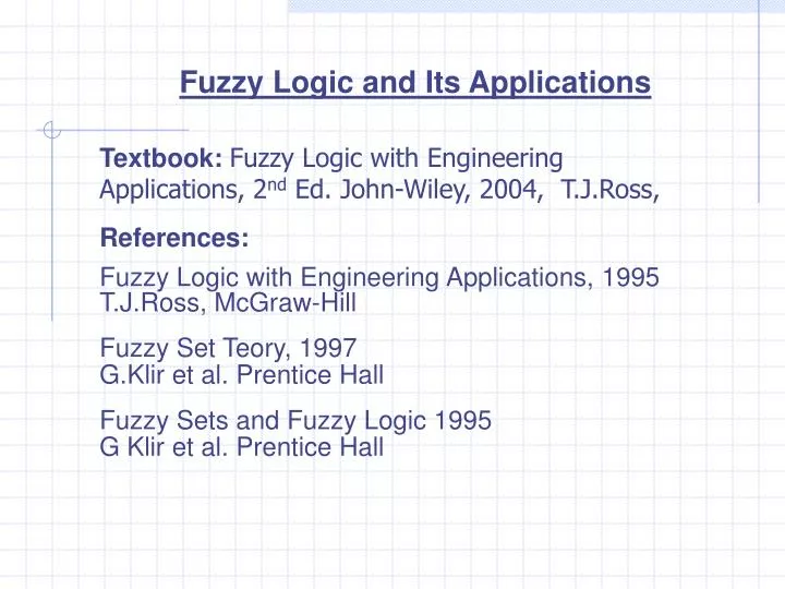
Fuzzy Logic and Its Applications. Textbook: Fuzzy Logic with Engineering Applications, 2 nd Ed. John-Wiley, 2004, T.J.Ross, References: Fuzzy Logic with Engineering Applications, 1995 T.J.Ross, McGraw-Hill Fuzzy Set Teory, 1997 G.Klir et al. Prentice Hall Fuzzy Sets and Fuzzy Logic 1995

E N D
Fuzzy Logic and Its Applications Textbook: Fuzzy Logic with Engineering Applications, 2nd Ed. John-Wiley, 2004, T.J.Ross, References: Fuzzy Logic with Engineering Applications, 1995 T.J.Ross, McGraw-Hill Fuzzy Set Teory, 1997 G.Klir et al. Prentice Hall Fuzzy Sets and Fuzzy Logic 1995 G Klir et al. Prentice Hall
Introduction In 1965, Prof. Lofti Zadeh published the first article “Fuzzy Sets”. It becomes billions of dollars business. America Europe Asia Thousands of patents Uncertainty: Incomplete Ambiguity: Imprecise Applications: Air Conditioner Washing Machine Subway System Camera Aerospace Nuclear Submarine Pattern Recognition Control Image Processing Computer Vision
They reflect a recent trend to view fuzzy logic (FL), neurocomputing (NC), genetic computing (GC), Rough Sets (RS) and probabilistic computing (PC) as an association of computing methodologies falling under the rubric of so-called soft computing. Among the basic concepts that underlie human cognition, three stand out in importance: granulation, organization, and causation.
Granulation involves a partitioning of a whole into parts; organization involves an integration of parts into a whole; and causation relates to an association of causes with effects A granule may be viewed as a clump of points (objects) drawn together by indistinguishability, similarity, or functionality. Modes of information granulation (IG) in which granules are crisp play an important role in many theories, methods and techniques, among them interval analysis, quantization, rough set theory, qualitative process theory, and chunking.
In fuzzy logic, fuzzy IG underlies the basic concepts of linguistic variables, fuzzy if-then rules, and fuzzy graphs This perception is reinforced by viewing it in the context of generalization. More specifically, any theory, method, technique, or problem may be fuzzified (or f-generalized) by replacing the concept of a crisp set with that of a fuzzy set. Similarly, any theory, method, technique, or problem can be granulated (g-generalized) by partitioning variables, functions, and relations into granules.
Furthermore, we can combine fuzzification with granulation, which gives rise to fuzzy granulation (f-granulation). Fuzzy granulation, then, provides a basis for what might be called f.g-generalization. The generalization of two-valued logic leads to multivalued logic and parts of fuzzy logic. But fuzzy logic in its wide sense—which is the sense in which it is used today—results from f.g-generalization. This crucial difference between multivalued logic and fuzzy logic explains why fuzzy logic has so many applications, whereas multivalued logic does not.
Introduction Fuzzy set theory provides a means for representing uncertainties. Probablity – random uncertainty But some uncertainty is non-random In fact, a huge amount! Natural Language is vague and imprecise. Fuzzy set theory uses Linguistic variables, rather than quantitative variables to represent imprecise concepts.
Fuzzy Logic Fuzzy Logic is suitable to Very complex models Judgemental Reasoning Perception Decision making Requiring precision – high cost, long time Statistics and random processes Based on Randomness.
Fuzziness Example. Random Errors generally average out over time or space Non-random errors will not generally average out and likely to grow with time. Information World
Information World Crisp set has a unique membership function A(x) = 1 x A 0 x A A(x) {0, 1} Fuzzy Set can have an infinite number of membership functions A [0,1]
Fuzziness Examples: A number is close to 5
Fuzziness Examples: He/she is tall
Fuzziness Randomness versus Fuzziness Drinking Water Problem Classical Sets Fuzzy Sets
Operations on Classical Sets Union: A B = {x | x A or x B} Intersection: A B = {x | x A and x B} Complement: A’ = {x | x A, x X} X – Universal Set Set Difference: A | B = {x | x A and x B} Set difference is also denoted by A - B
Properties of Classical Sets A B = B A A B = B A A (B C) = (A B) C A (B C) = (A B) C A (B C) = (A B) (A C) A (B C) = (A B) (A C) A A = A A A = A A X = X A X = A A = A A =
Properties of Classical Sets If A B C, then A C De Morgan’s Law: (A B)’ = A’ B’ (A B)’ = A’ B’ Proof: LHS= {x | x (A and B)}= {x | x A or x B)}= A’ B’= RHS
Can be extended to n sets Generalized De Morgan Law: A A’ X X Using ( ) to keep original processing order
Generalized Duality Law: X X Using ( ) to keep original processing order
Law of the excluded middle: A A’ = X Law of the Contradiction: A A’ = These laws are not true for Fuzzy Sets!
Fuzzy Sets Characteristic function X, indicating the belongingness of x to the set A X(x) = 1 x A 0 x A or called membership Hence, A B XA B(x) = XA(x) XB(x) = max(XA(x),XB(x)) Note:Some books use + for , but still it is not ordinary addition! Some more explanations follow…
Fuzzy Sets A B XA B(x) = XA(x) XB(x) = min(XA(x),XB(x)) A’ XA’(x) = 1 – XA(x) A B XA(x) XB(x) A’’ = A
Fuzzy Sets Note (x) [0,1] not {0,1} like Crisp set A = {A(x1) / x1 + A(x2) / x2 + …} = { A(xi) / xi} Note: ‘+’ add ‘/ ’ divide Only for representing element and its membership. Also some books use (x) for Crisp Sets too.
Fuzzy Set Operations A B(x) = A(x) B(x) = max(A(x), B(x)) A B(x) = A(x) B(x) = min(A(x), B(x)) A’(x) = 1 - A(x) De Morgan’s Law also holds: (A B)’ = A’ B’ (A B)’ = A’ B’ But, in general A A’ A A’
Properties of Fuzzy Sets A B = B A A B = B A A (B C) = (A B) C A (B C) = (A B) C A (B C) = (A B) (A C) A (B C) = (A B) (A C) A A = A A A = A A X = X A X = A A = A A = If A B C, then A C A’’ = A
Sets as Points in Hypercubes Explore to n-dimension Classical Relations Fuzzy relations Logic, Approximate reasoning, Rule-based learning systems, Nonlinear Simulation, Classification, Pattern Recognition, etc.
Cartesian Product A = {a,b} B = {0,1} A x B = { (a,0) (a,1) (b,0) (b,1) } Ordered Pairs Consider A x A or A x B x C if C is given Based on the above, Crisp Relations are discussed next…
Crisp Relations A subset of a Cartesian Product A1 x A2 x … x Ar is called an r-ary relation over A1,A2,…,Ar If r = 2, the relation is a subset of A1 x A2 Binary relation from A1 into A2 The strength of a relation: Characteristic Function X(x,y) = 1 (x,y) X x Y 0 (x,y) X x Y For Classical relations, the value is 1 or 0 If the universes or sets are finite, we can use relational matrix to represent it.
Crisp Relations Example: If X = {1,2,3} Y = {a,b,c} R = { (1 a),(1 c),(2 a),(2 b),(3 b),(3 c) } a b c 1 1 0 1 R = 2 1 1 0 3 0 1 1 Using a diagram to represent the relation
Crisp Relations Relations can also be defined for continuous universes R = { (x,y) | y 2x, x X, y Y} X = 1 y 2x 0 otherwise
Crisp Relations Cardinality: N: # of elements in X M: # of elements in y Cardinality of R nX x Y = nX• nY = M • N Cardinality of the Power set of this relation nP(X x Y) = 2MN
Operations on Crisp Relations • Complete Relation Matrix • 1 1 1 • 1 1 • 1 1 1 • Null relation Matrix • 0 0 0 • 0 0 0 • 0 0 0
Operations on Crisp Relations Union R S XR S(x,y) XR S(x,y) = max{ XR(x,y),XS(x,y) } Intersection R S XR S(x,y) XR S(x,y) = min{ XR(x,y),XS(x,y) } Complement R’ XR’(x,y) XR’(x,y) = 1 – XR(x,y) Containment R S XR(x,y) XS(x,y) Identity 0 X E
Properties of Crisp Relations Commutativity Associativity Distributivity Idempotency All hold De Morgan Law Excluded middle Law Etc.
Properties of Crisp Relations Composition Let R be a relation representing a mapping from X to Y X Y University sets Let S be a relation, a mapping from Y to Z Can we find T from R to S?
Properties of Crisp Relations • T: mapping from X to Z • T = R S • Two ways to compute XT(xz) • XT(xz) = (XR(xy) Xs(yz)) • = max(min{XR(xy),XS(yz)}) • Max-min composition • XT(xz) = (XR(xy) Xs(yz)) • Max-product composition • multiplication y Y y Y y Y
Properties of Crisp Relations Using Matrix representation: y1 y2 y3 y4 x1 1 0 1 0 R = x2 0 0 0 1 x3 0 0 0 0 z1 z2 y1 0 1 z1 z2 y2 0 0 x1 0 0 S = y3 0 1 T = x2 0 0 y4 0 0 x3 0 0 T(x1,z1) = max[min(1,0) min(0,0) min(1,0) min(0,0)] = max[0,0,0,0] = 0 Similar, but not the same as matrix multiplication!
Fuzzy Relations Cardinality of Fuzzy Relations Since the cardinality of fuzzy sets on any universe is infinity, the cardinality of a fuzzy relation is also infinity. Note: other books have different discussions!
Operations on Fuzzy Relations Union: R S = max{ R(x,y),S(x,y) } Intersection: R S = min{ R(x,y),S(x,y) } Complement: R’(x,y) = 1 - R(x,y) Containment: R S R(x,y) S(x,y)
Properties of Fuzzy Relations Commutativity Associativity Distributivity Idempotency All hold De Morgan Law Excluded middle Law Etc. Note: R R’ E R R’ 0 In general.
Properties of Fuzzy Relations Fuzzy Cartesian Product and Composition R(x y) = A x B(x y) = min(A(x), B(y)) Example: A = 0.2/x1 + 0.5/x2 + 1/x3 B = 0.3/y1 + 0.9/y2 y1 y2 0.2 x1 0.2 0.2 A x B = 0.5 0.3 0.9 = x2 0.3 0.5 1 x3 0.3 0.9
Properties of Fuzzy Relations • Vector Outer Product • If R is a fuzzy relation on the space X x Y • S is a fuzzy relation on the space Y x Z • Then, fuzzy composition is T = R S • Fuzzy max-min composition • T(xz) = (R(xy) s(yz)) • 2. Fuzzy max-production composition • T(xz) = (R(xy) s(yz)) • Note:R S S R y Y y Y
Properties of Fuzzy Relations Example: y1 y2 z1 z2 z3 R = x1 0.7 0.5 S = y1 0.9 0.6 0.2 x2 0.8 0.4 y2 0.1 0.7 0.5 z1 z2 z3 Using max-min, T = x1 0.7 0.6 0.5 x2 0.8 0.6 0.4 z1 z2 z3 Using max-product, T = x1 0.63 0.42 0.25 x2 0.72 0.48 0.20 Note: Set, Relation, Composition How to find new membership from the given ones!
Tolerance and Equivalence Relation Crisp Equivalence Relation R X x X Relation has the following properties: Reflexivity (xi xi) R or XR(xi xi) = 1 Symmetry (xi xj) R (xj xi) R or XR(xi xj) = XR(xj xi) Transitivity (xi xj) R and (xj xk) R (xi xk) R or XR(xi xj) = 1 and XR(xj xk) = 1 XR(xi xk) = 1
Tolerance and Equivalence Relation Graph representation:
Crisp Tolerance Relation (or proximity relation) Only has reflexivity and symmetry A tolerance relation, R1 can become an Equivalence Relation by at most (n-1) compositions ( n-1), n is the cardinal member of X. R1n-1 = R1 R1 … R1 = R
Crisp Tolerance Relation (or proximity relation) Example: 1 1 0 0 0 1 1 0 0 1 R1 = 0 0 1 0 0 0 0 0 1 0 0 1 0 0 1 1 1 0 0 1 1 1 0 0 1 Try R12 = 0 0 1 0 0 0 0 0 1 0 1 1 0 0 1 Note: symmetric, reflexive, but not transitive, why? X(x1 x2) = 1 X(x2 x5) = 1 but X(x1 x5) 1 (=0) Now, it is transitive!
Fuzzy Tolerance and Equivalence Relation A fuzzy relation R has: 1. Reflexivity R(xi xi) = 1 2. Symmetry R(xi xj) = R(xj xi) 3. Transitivity R(xi xj) = 1 R(xj xk) = 2 R(xi xk) = where min{1, 2} Fuzzy tolerance relation R1 has reflexivity, symmetry. It can be transformed into a fuzzy equivalence relation by at most (n-1) ( n-1) compositions. R1n-1 = R1 R1 … R1 = R
Fuzzy Tolerance and Equivalence Relation Example: 1 0.8 0 0.1 0.2 0.8 1 0.4 0 0.9 R1 = 0 0.4 1 0 0 0.1 0 0 1 0.5 0.2 0.9 0 0.5 1 R1(x1 x2) = 0.8 R1(x2 x5) = 0.9 But R1(x1 x5) = 0.2 min(0.8,0.9) not transitive
Fuzzy Tolerance and Equivalence Relation • Value Assignment • How to find the membership values for the relation? • Cartesian Production • Note: you have to know the membership value for the sets! Will discuss in chapter 4. • 2. Y = f(x) X – input vector • Y – output vector • 3. Look up table y1 y2 y3 • x1 • x2 • x3
Fuzzy Tolerance and Equivalence Relation Value Assignment 4. Linguistic rule of knowledge – chapters 7 – 9 5. Classification – chapter 11 6. Similarity methods in data manipulation The more robust a data set, the more accurate the relation entries!