Hypothesis Testing Large Samples
Hypothesis Testing Large Samples

Hypothesis Testing Large Samples
E N D
Presentation Transcript
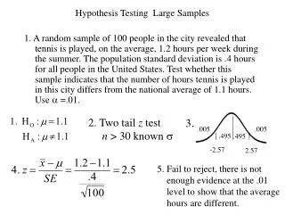
Hypothesis Testing Large Samples 1. A random sample of 100 people in the city revealed that tennis is played, on the average, 1.2 hours per week during the summer. The population standard deviation is .4 hours for all people in the United States. Test whether this sample indicates that the number of hours tennis is played in this city differs from the national average of 1.1 hours. Use =.01. 3. 2. Two tail z test n > 30 known .005 .005 .495 .495 -2.57 2.57 5. Fail to reject, there is not enough evidence at the .01 level to show that the average hours are different.
Hypothesis Testing Large Samples 2. The population of all minority workers has a mean wage of $14,500 with a standard deviation of $200.00. Test whether a sample of 100 having an average of $14,300 and = .05 differs from the population average. 3. 2. Two tail z test n > 30 known .025 .025 .475 .475 1.96 -1.96 5. Reject HO at the .05 level. There is evidence that the salaries are different.
Hypothesis Testing Large Samples 3. A new bus route has been established. For the old route, the average waiting time was 18.3 minutes. However, a random sample of 40 waiting times between buses using the new route had a mean of 15.1 minutes with a sample standard deviation of 6.2 minutes. Does this indicate that the new route is different from the old route? Use = .05. 3. 2. Two tail z test n > 30 .025 .025 .475 .475 1.96 -1.96 5. Reject HO at the .05 level. There is evidence that the new route is different.
Hypothesis Testing Small Samples 1. A manufacturer of ball bearings have a diameter of .25 inches and a sample standard deviation of .05 inches. A random sample of n = 25 ball bearings reveal a mean diameter of .2670 inches. Conduct a hypothesis test at the 10 % level of significance to determine whether there is statistical significance that the manufacturing process is not running correctly, that is µ ≠ .25 inches. 3. 2. Two tail t test n < 30 unknown 24 d.f. .05 .05 -1.711 1.711 5. Fail to reject HO at the .1 level. There is not enough evidence that it is not running incorrectly.
Hypothesis Testing Small Samples 2. A random sample of n = 10 prices of CDs gives the following values: $24.19, $21.04, $12.34, $16.07, $19.65, $19.36, $15.99, $15.02. $18.68, $20.60. Conduct a hypothesis test at the 10% level to determine whether evidence exists to support the claim that the population average is less than $19.00. 3. 2. One tail t test n < 30 unknown 9 d.f. .01 -1.383 5. Fail to reject HO at the .1 level. There is not evidence that average CD price is less than $19.00.
Hypothesis Testing Large Sample Population Proportion 1. A telephone survey was conducted to determine viewer response to a new show. The sponsor would like to see a favorable response from over 65% of the respondents. From a sample of 500 viewers, 345 of the responses were favorable. Is there sufficient evidence to satisfy the sponsor at the .01 level? 3. 2. One tail z test (500)(.65) > 5 (500)(.35) > 5 .01 2.33 5. Fail to reject HO at the .1 level. There is not enough evidence to satisfy the sponsor.
Hypothesis Testing Difference of Population Means 1. In a certain industry, the standard deviation for workers in Chicago is the same as in Los Angeles = $2.75 per hour. A random sample of 30 workers in Chicago revealed a mean wage of $22.75 per hour and a random sample of 40 from Los Angeles revealed a mean wage of $18.55 per hour. Perform a hypothesis test at the .01 significance level to determine whether they are different and construct an 80 % confidence interval. 2. Two tail z test nC, nL > 30 3. .005 .005 -2.58 2.58 5. Reject HO at the .1 level, the wages are different 4.2 + 1.28(.66) (3.35, 5.04)
Hypothesis Testing Difference of Population Means 2. In a study of heart surgery, the effect of a beta-blocker was used to reduce pulse rate. One group of 30 received the drug and had an average pulse rate of 65.2 beats per minute and a standard deviation of 7.8. For the control group of 30 which received the placebo, the mean was 70.3 beats per minute with a standard deviation of 8.3. Do beta-blockers reduce pulse rate? Is the result significant at the .05 level? Construct a 99% confidence interval for the difference in mean pulse rate. 3. 2. One tail z test nB, nP > 30 .05 -1.645 5. Reject HO at the .05 level, beta blockers reduce blood pressure -5.1 + 2.58(2.07) (-10.46, .26)
Hypothesis Testing Difference of Population Means 2. The prices for a certain drug at a private and a chain drug store are shown. Perform a hypothesis test at the .01 level to determine if the prices are different. 3. 2. Two tail t test 22 d.f. .005 -2.82 2.82 5. Fail to reject HO at the .01 level, no difference in prices.
Hypothesis Testing Difference of Population Means 1. Two groups of infants were compared with the amount of blood hemoglobin levels at 12 months of age. Is there evidence at the .01 level that the two methods are different. Give a 95% confidence interval between the two populations of infants. 3. 2. Two tail t test 40 d.f. .005 -2.70 2.70 5. Reject HO at the .1 level, no difference in feeding methods. .9 + 1.96(.54) (-.158, 1.958)
pd = 56/2051=.027 pp = 84/2030=.041 Hypothesis Testing Difference of Population Proportions 1. A sample of 2051 men taking a drug to reduce heart attacks had 56 heart attacks during the next five years while a sample of 2030 resulted in 84 heart attacks during the next 5 years. Is there evidence at the .01 level that the drug reduces the possibility of a heart attack? 3. 2. One tail z test .01 -2.33 5. Reject HO at the .1 level, the drug reduces heart attacks.
Hypothesis Testing Difference of Population Proportions 2. A sample of 267 white people and 230 black people were asked if the government was doing enough in the areas of housing, unemployment, and education. 161 of the white people surveyed and 136 of the black people said no. Is there evidence at the .05 level that the white people and black people disagree on this issue? p1 = 161/267=.60 p2 = 136/230=.59 3. 2. Two tail z test .025 .025 -1.96 1.96 5. Fail to reject HO at the .05 level, there is no difference between voting preference.
Hypothesis Testing Matched Pair Samples 1. Cola makers test new recipes for loss of sweetness before and after storage. The results of ten tasters are shown before and after storage. Is their evidence at the .05 level that sweetness is greater before storage? 3. .05 2. One tail t test 9 d.f. 1.83 5. Reject HO at the .05 level, sweetness is greater before storage
Hypothesis Testing Matched Pair Samples 2. A physical education teacher tested the results of jogging on a person’s cardiovascular system. The resting pulse rates were measured before and after the completion of a 5 week jogging program. Is there evidence at the .01 level that the resting pulse rate decreased? .01 3. 2. One tail t test 6 d.f. -3.14 5. Reject HO at the .01 level, the resting pulse rate decreased
Hypothesis Testing Chi Square The following table shows the results of boys and Girls that get in trouble in school. Are gender and getting in trouble independent at the .01 level?
6.64 • HO: Gender and trouble are independent HA: Gender and trouble are dependent 2. Chi Square test (2 - 1)(2 - 1) = 1 d.f. 3. Determine rejection region 4. Compute test statistic 1.87 5. Fail to Reject HO, gender and trouble are not independent
The following table shows the Myers-Brigs personality preference and professions for a random sample of 2408 people in the listed professions. E refers to extroverted and I refers to introverted. Use the chi-squared test to determine if the listed occupations and personality preferences are independent at the .01 level of significance.
534 293 241 1603 879 723 271 149 122 1321 1087 2408 Use the chi-squared test to determine if the listed occupations and personality preferences are independent at the .01 level of significance.
9.21 • HO: Preferences and profession are independent HA: Preferences and profession are dependent 2. Chi Square test (3 - 1)(2 - 1) = 2 d.f. 3. Determine rejection region 4. Compute test statistic 43.55 = 43.55 5. Reject HO, preferences and profession are not independent