Download
1 / 5
50 likes | 142 Views

E N D
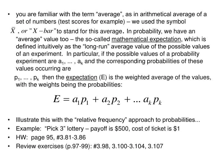
you are familiar with the term “average”, as in arithmetical average of a set of numbers (test scores for example) – we used the symbol to stand for this average.In probability, we have an “average” value too – the so-called mathematical expectation, which is defined intuitively as the “long-run” average value of the possible values of an experiment. In particular, if the possible values of a probability experiment are a1, ... , ak and the corresponding probabilities of these values occurring are p1, ... , pk then the expectation (E) is the weighted average of the values, with the weights being the probabilities: • Illustrate this with the “relative frequency” approach to probabilities... • Example: “Pick 3” lottery – payoff is $500, cost of ticket is $1 • HW: page 95, #3.81-3.86 • Review exercises (p.97-99): #3.98, 3.100-3.104, 3.107
We are going to be concerned with random variables, a function that assigns a numerical value to each possible outcome of a random experiment • X=sum of spots when a pair of fair dice is thrown • Y=# of Hs that come up when a fair coin is tossed 4 times. • We are going to be interested in the probability distribution of the random variable (rv): i.e., the list of all the possible values of the rv and the corresponding probabilities that the variable takes on those values... get the probability distributions of the two example rvs X and Y above... • If we write f(x) = P(X = x) then it must be the case that
We will be considering several discrete random variables and their distributions • Binomial: X = the number of S’s in n Bernoulli trials (recall Bernoulli trials or see p. 105)... our previous rv counting the number of Hs in 4 tosses of a fair coin is a typical Binomial variable – we denote the binomial probabilities by • Cumulative binomial probabilities are given in Table 1 for various values of n and p; write • TI-83 can do binomial probabilities under 2nd VARS binompdf (individual binomial probs) or binomcdf (cumulative binomial probs) • R can calculate binomial probabilities (see the R handout)
we can think about the binomial rv as “sampling with replacement” (Hs and Ts in equal numbers in an urn, replace after each draw...). The hypergeometric rv can be thought about in the same way except that the sampling is to be done “without replacement” from an urn with N items, a Ss and N-a Fs. • Lot of 20 items, 5 defective (“success”). Choose 10 at random; what is the probability that exactly 2 of the 10 are defective? Ans: h(2; 10, 5, 20) = .348 NOTE: This can be approximated by b(2; 10, .25) = .282 (not so good...but if the N were larger... what would happen?)
Example (p.111) N=100, a=25 (so p remains .25): then h(2; 10, 25, 100) = .292 and b(2; 10, .25) = .282 • The mathematical result is that as N approaches infinity with p=a/N, h(x; n, a, N) approaches b(x; n, p) and a good rule of thumb is to use the binomial if n <= N/10 • HW: Read sections 4.1-4.3; work on problems # 4.2, 4.3, 4.5, 4.7, 4.9, 4.13, 4.17, 4.19, 4.20, 4.21, 4.23, 4.25, 4.28, 4.29