Download

1 / 20
200 likes | 367 Views
Analysis of Variance and Multiple Comparisons. Comparing more than two means and figuring out which are different. Analysis of Variance (ANOVA). Despite the name, the procedures compares the means of two or more groups Null hypothesis is that the group means are all equal

E N D
Analysis of Variance and Multiple Comparisons Comparing more than two means and figuring out which are different
Analysis of Variance (ANOVA) • Despite the name, the procedures compares the means of two or more groups • Null hypothesis is that the group means are all equal • Widely used in experiments, it is less common in anthropology
ANOVA in Rcmdr • Statistics | Means | One-way ANOVA • Accept or change the model name • Select a group (only factors are listed here) • Select a response variable (only numeric variables are listed here) • Check Pairwise comparison of means
> AnovaModel.1 <- aov(Area ~ Segment, data=Snodgrass) > summary(AnovaModel.1) Df Sum Sq Mean Sq F value Pr(>F) Segment 2 432327 216164 51.817 1.344e-15 *** Residuals 88 367107 4172 --- Signif. codes: 0 '***' 0.001 '**' 0.01 '*' 0.05 '.' 0.1 ' ' 1 > numSummary(Snodgrass$Area , groups=Snodgrass$Segment, + statistics=c("mean", "sd")) mean sd n 1 317.3711 76.08797 38 2 166.7946 59.99526 28 3 192.7900 48.18188 25
Results • Since the ANOVA statistic is less than our critical value (.05), we reject the null hypothesis that the mean Areas of Segments 1 = 2 = 3 • But we usually want to know more • Since we did not make predictions in advance our comparisons are post hoc
Multiple Comparisons • To find out which means are different from each other we have to compare the various combinations: 1 with 2, 1 with 3, and 2 with 3 • (we could also perform other comparisons such as 1 and 2 with 3 but they are rare in anthropology
More Kinds of Errors • Our statistical tests have focused on setting the Type I error rate at .05 – the comparisonwise error rate • But this error rate holds for a single test. If we do many tests, the chance that we will commit at least one Type 1 error will be higher – the experimentwise error rate
Calculating Errors • If the probability of a Type I error is .05, the probability of not making a Type I error is (1 - .05) = .95 • The probability of not making a Type I error twice is .952 = .9025, three times - .953 = .8574, four times - .954 = .8145
Calculating Errors • The probability of making at least one Type I error is • Twice – (1 - .9025) = .0975 • Thrice – (1 - .8574) = .1426 • Four times – (1 - .8145) = .1855 • The probability of making at least one Type I error increases with each additional test
curve((1-(1-.05)^x), 1, 50, 50, yaxp=c(0, .9, 9), xaxp=c(0, 50, 10), xlab="Number of Comparisons", ylab="Type I Error Rate", las=1, main="Experimentwise Error Rate") curve((1-(1-.01)^x), 1, 50, 50, lty=2, add=TRUE) text(30, .92, expression(p == 1-(1-.05)^x), pos=4) text(30, .37, expression(p == 1-(1-.01)^x), pos=4) abline(h=seq(.1, .9, .1), v=seq(0, 50, 5), lty=3, col="gray") legend("topleft", c("Comparisonwise p = .05", "Comparisonwise p = .01"), lty=c(1, 2), bg="white")
Multiple Comparisons • Multiple Comparisons procedures take experimentwise error into account when comparing the group means • There are a number of methods available, but we’ll stick with Tukey’s Honestly Significant Differences (aka Tukey’s range test)
Tukey’s HSD • One of the few multiple comparison tests that can adjust for different sample sizes among the groups • You requested this test in Rcmdr when you checked “Pairwise comparison of the means”
> .Pairs <- glht(AnovaModel.1, linfct = mcp(Segment = "Tukey")) > summary(.Pairs) # pairwise tests Simultaneous Tests for General Linear Hypotheses Multiple Comparisons of Means: Tukey Contrasts Fit: aov(formula = Area ~ Segment, data = Snodgrass) Linear Hypotheses: Estimate Std. Error t value Pr(>|t|) 2 - 1 == 0 -150.58 16.09 -9.361 <1e-04 *** 3 - 1 == 0 -124.58 16.63 -7.490 <1e-04 *** 3 - 2 == 0 26.00 17.77 1.463 0.313 --- Signif. codes: 0 '***' 0.001 '**' 0.01 '*' 0.05 '.' 0.1 ' ' 1 (Adjusted p values reported -- single-step method)
> confint(.Pairs) # confidence intervals Simultaneous Confidence Intervals Multiple Comparisons of Means: Tukey Contrasts Fit: aov(formula = Area ~ Segment, data = Snodgrass) Quantile = 2.383 95% family-wise confidence level Linear Hypotheses: Estimate lwrupr 2 - 1 == 0 -150.5764 -188.9093 -112.2435 3 - 1 == 0 -124.5811 -164.2161 -84.9460 3 - 2 == 0 25.9954 -16.3553 68.3460
NonParametric ANOVA • The non-parametric alternative to ANOVA is the Kruskal-Wallis Rank Sum Test • The null hypothesis is that the medians of the groups are equal • If the test is significant, a multiple comparison method is available to identify which groups are different
Kruskal-Wallis in Rcmdr • Statistics | Nonparametric tests | Kruskal-Wallis test • Select a group (only factors are listed here) • Select a response variable (only numeric variables are listed here)
Multiple Comparisons • If there are significant differences the function kruskalmc() in package pgirmess will tell you what groups are different
> kruskal.test(Area ~ Segment, data=Snodgrass) Kruskal-Wallis rank sum test data: Area by Segment Kruskal-Wallis chi-squared = 50.4427, df = 2, p-value = 1.113e-11 library(pgirmess) > kruskalmc(Area ~ Segment, data=Snodgrass) Multiple comparison test after Kruskal-Wallis p.value: 0.05 Comparisons obs.dif critical.dif difference 1-2 43.125940 15.74873 TRUE 1-3 35.227368 16.28369 TRUE 2-3 7.898571 17.39936 FALSE