MATLAB Post-Processing Techniques: Vectors, Graphics, and Analytical Solutions
This MATLAB guide covers post-processing techniques for vectors, matrices, graphics, and analytical solution comparisons. Learn how to manipulate vectors, create xy plots, work with matrices, reshape data, load files, use loops and conditions, generate BMP outputs, plot contours, and visualize data using quiver and streamline plots. Dive into advanced techniques like generating streamlines with custom starting points to analyze complex fluid dynamics simulations.


MATLAB Post-Processing Techniques: Vectors, Graphics, and Analytical Solutions
E N D
Presentation Transcript
-
Matlab • Post-processer • Graphics • Analytical solution comparisons
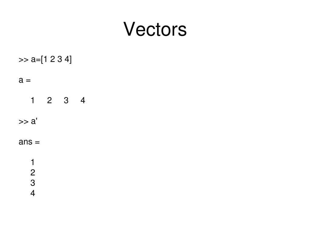
Vectors >> a=[1 2 3 4] a = 1 2 3 4 >> a' ans = 1 2 3 4
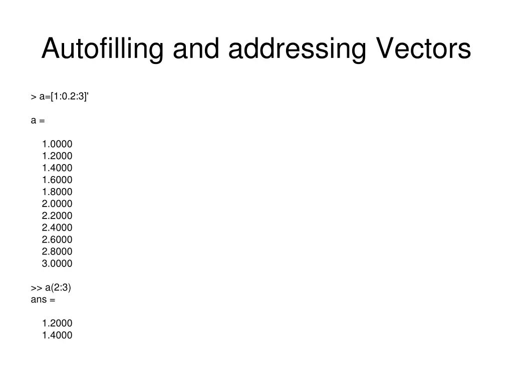
Autofilling and addressing Vectors > a=[1:0.2:3]' a = 1.0000 1.2000 1.4000 1.6000 1.8000 2.0000 2.2000 2.4000 2.6000 2.8000 3.0000 >> a(2:3) ans = 1.2000 1.4000
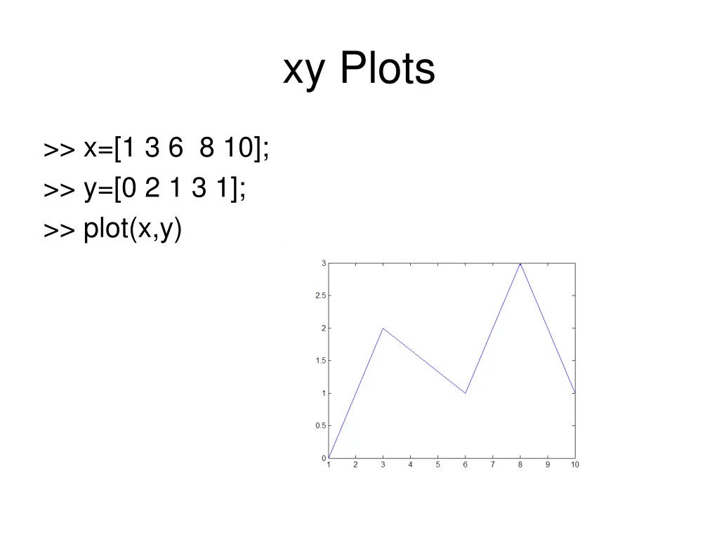
xy Plots >> x=[1 3 6 8 10]; >> y=[0 2 1 3 1]; >> plot(x,y)
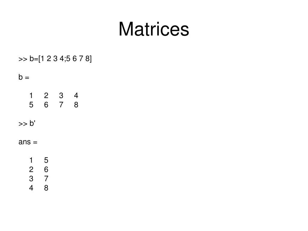
Matrices >> b=[1 2 3 4;5 6 7 8] b = 1 2 3 4 5 6 7 8 >> b' ans = 1 5 2 6 3 7 4 8
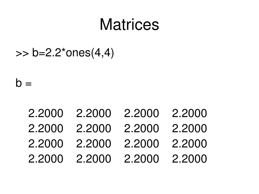
Matrices >> b=2.2*ones(4,4) b = 2.2000 2.2000 2.2000 2.2000 2.2000 2.2000 2.2000 2.2000 2.2000 2.2000 2.2000 2.2000 2.2000 2.2000 2.2000 2.2000
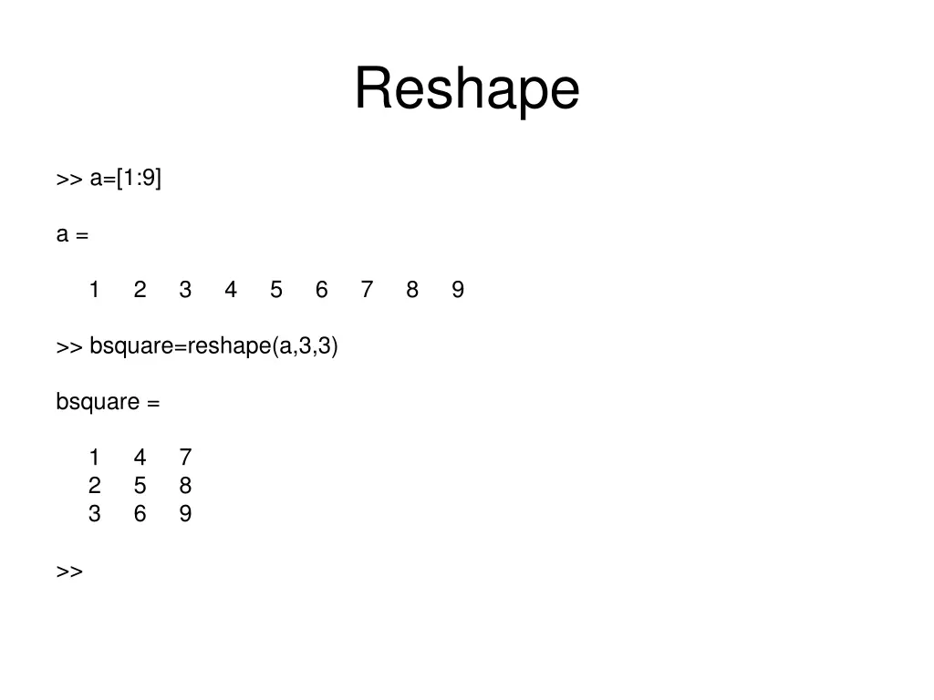
Reshape >> a=[1:9] a = 1 2 3 4 5 6 7 8 9 >> bsquare=reshape(a,3,3) bsquare = 1 4 7 2 5 8 3 6 9 >>
Load and if • a = load(‘filename’); (semicolon suppresses echo) • if(1) … else … end
For • for i = 1:10 • … • end
Grad [dhdx,dhdy]=gradient(h);
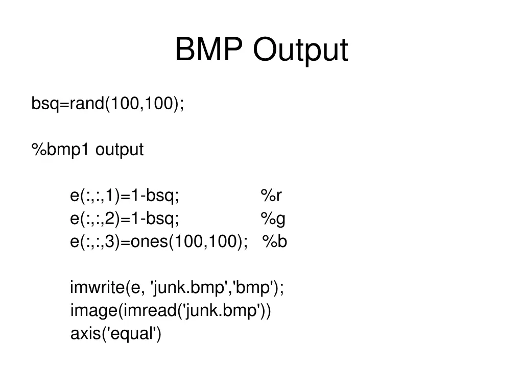
BMP Output bsq=rand(100,100); %bmp1 output e(:,:,1)=1-bsq; %r e(:,:,2)=1-bsq; %g e(:,:,3)=ones(100,100); %b imwrite(e, 'junk.bmp','bmp'); image(imread('junk.bmp')) axis('equal')
Contours • h=[…]; • contour(h) • [C,H]=contour(h) • Clabel(C,H)
Contours (load data, prepare matrix) rho=load('rho_frame0012_subs00.dat') p_vector=rho/3 rows=100 columns=20 • • • • for j=1:columns j for i=1:rows p(i,j)=p_vector(j+(i-1)*columns); • • • • • • • • • • • %Get rid of '0 pressure' solids that dominate pressure field if p(i,j)==0 p(i,j)=NaN; end end end
Contours • [C,H]=contour(p) • clabel(C,H) • axis equal
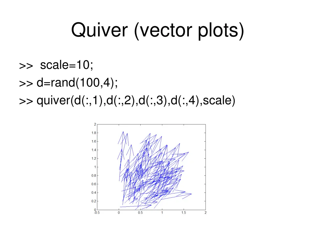
Quiver (vector plots) >> scale=10; >> d=rand(100,4); >> quiver(d(:,1),d(:,2),d(:,3),d(:,4),scale)
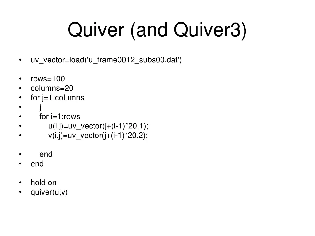
Quiver (and Quiver3) uv_vector=load('u_frame0012_subs00.dat') • rows=100 columns=20 for j=1:columns j for i=1:rows u(i,j)=uv_vector(j+(i-1)*20,1); v(i,j)=uv_vector(j+(i-1)*20,2); • • • • • • • end • • end hold on quiver(u,v) • •
Streamline • [Stream]= stream2(u,v,5,100) • streamline(Stream)
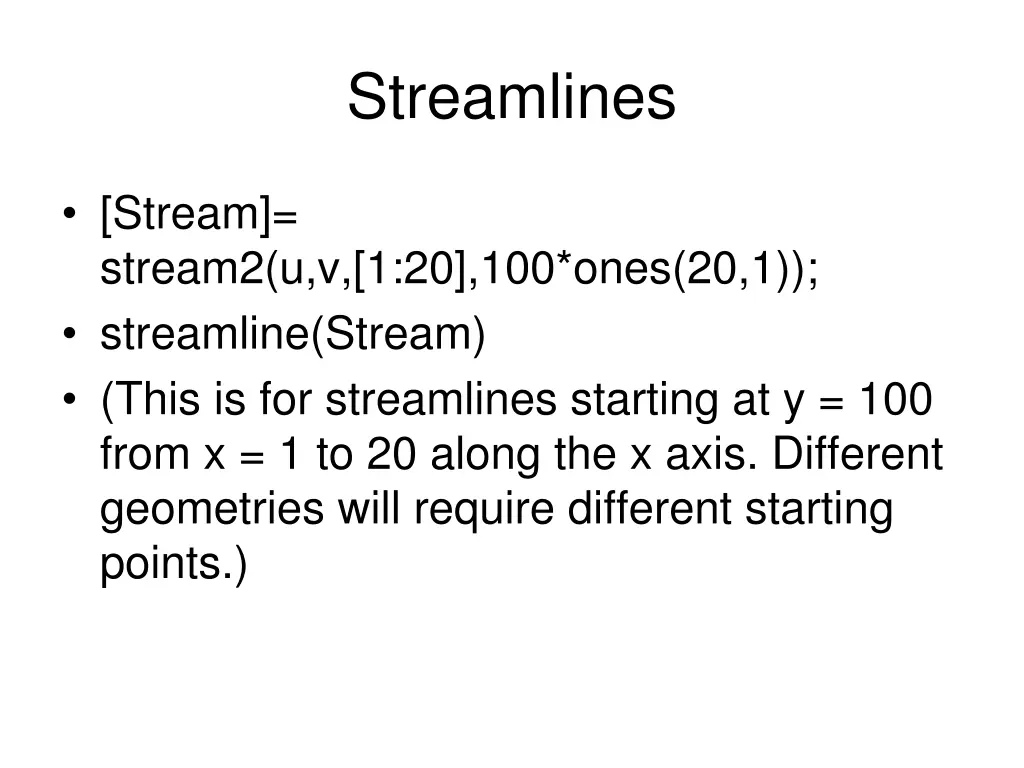
Streamlines • [Stream]= stream2(u,v,[1:20],100*ones(20,1)); • streamline(Stream) • (This is for streamlines starting at y = 100 from x = 1 to 20 along the x axis. Different geometries will require different starting points.)