Inflation
27. Inflation. CHAPTER. Objectives. After studying this chapter, you will able to Distinguish between inflation and a change in the price level and between demand-pull inflation and cost-push inflation Explain the quantity theory of money


Inflation
E N D
Presentation Transcript
27 Inflation CHAPTER
Objectives • After studying this chapter, you will able to • Distinguish between inflation and a change in the price level and between demand-pull inflation and cost-push inflation • Explain the quantity theory of money • Explain the short-run and long-run relationships between inflation and unemployment • Explain the short-run and long-run relationships between inflation and interest rates
From Rome to Rio de Janeiro • Inflation is a very old problem and some countries even in recent times have experienced rates as high as 40 percent a month. • Today, the Bank of Canada targets the inflation rate and keeps it low. But during the 1970s, the price level in Canada doubled. • Why does inflation occur and do our expectations of inflation influence the economy? • In targeting inflation, does the Bank of Canada face a tradeoff between inflation and unemployment? And how does inflation affect the interest rate?
Inflation: Demand-Pull and Cost-Push • Inflation is a process in which the price level is rising and money is losing value. • Inflation is a rise in the price level, not in the price of a particular commodity. • And inflation is an ongoing process, not a one-time jump in the price level.
Inflation: Demand-Pull and Cost-Push • Figure 27.1 illustrates the distinction between inflation and a one-time rise in the price level.
Inflation: Demand-Pull and Cost-Push • The inflation rate is the percentage change in the price level. • That is, where P1 is the current price level and P0 is last year’s price level, the inflation rate is • [(P1 – P0)/P0] 100 • Inflation can result from either an increase in aggregate demand or a decrease in aggregate supply and be • Demand-pull inflation • Cost-push inflation
Inflation: Demand-Pull and Cost-Push • Demand-Pull Inflation • Demand-pull inflation is an inflation that results from an initial increase in aggregate demand. • Demand-pull inflation may begin with any factor that increases aggregate demand. • Two factors controlled by the government are increases in the quantity of money and increases in government purchases. • A third possibility is an increase in exports.
Inflation: Demand-Pull and Cost-Push • Initial Effect of an Increase in Aggregate Demand • Figure 27.2(a) illustrates the start of a demand-pull inflation. • Starting from full employment, an increase in aggregate demand shifts the AD curve rightward.
Inflation: Demand-Pull and Cost-Push • The price level rises, real GDP increases, and an inflationary gap arises. • The rising price level is the first step in the demand-pull inflation.
Inflation: Demand-Pull and Cost-Push • Money Wage Rate Response • Figure 27.2(b) illustrates the money wage response. • The money wages rises and the SAS curve shifts leftward. • Real GDP decreases back to potential GDP but the price level rises further.
Inflation: Demand-Pull and Cost-Push • A Demand-Pull Inflation Process • Figure 27.3 illustrates a demand-pull inflation spiral. • Aggregate demand keeps increases and the process just described repeats indefinitely.
Inflation: Demand-Pull and Cost-Push • Although any of several factors can increase aggregate demand to start a demand-pull inflation, only an ongoing increase in the quantity of money can sustain it. • Demand-pull inflation occurred in Canada during the late 1960s and early 1970s.
Inflation: Demand-Pull and Cost-Push • Cost-Push Inflation • Cost-push inflation is an inflation that results from an initial increase in costs. • There are two main sources of increased costs: • 1. An increase in the money wage rate • 2. An increase in the money price of raw materials, such as oil.
Inflation: Demand-Pull and Cost-Push • Initial Effect of a Decrease in Aggregate Supply • Figure 27.4 illustrates the start of cost-push inflation. • A rise in the price of oil decreases short-run aggregate supply and shifts the SAS curve leftward.
Inflation: Demand-Pull and Cost-Push • Real GDP decreases and the price level rises—a combination called stagflation. • The rising price level is the start of the cost-push inflation.
Inflation: Demand-Pull and Cost-Push • Aggregate Demand Response • The initial increase in costs creates a one-time rise in the price level, not inflation. • To create inflation, aggregate demand must increase.
Inflation: Demand-Pull and Cost-Push • Figure 27.5 illustrates an aggregate demand response to stagflation, which might arise because the Bank of Canada stimulates demand to counter the higher unemployment rate and lower level of real GDP. • Real GDP increases and the price level rises again.
Inflation: Demand-Pull and Cost-Push • A Cost-Push Inflation Process • Figure 27.6 illustrates a cost-push inflation spiral.
Inflation: Demand-Pull and Cost-Push • If the oil producers raise the price of oil to try to keep its relative price higher, • and the Bank of Canada responds with an increase in aggregate demand, • a process of cost-push inflation continues. • Cost-push inflation occurred in Canada during 1974–1978.
The Quantity Theory of Money • The quantity theory of money is the proposition that, in the long run, an increase in the quantity of money brings an equal percentage increase in the price level. • The quantity theory of money is based on the velocity of circulation and the equation of exchange. • The velocity of circulation is the average number of times in a year a dollar is used to purchase goods and services in GDP.
The Quantity Theory of Money • Calling the velocity of circulation V, the price level P, real GDP Y, and the quantity of money M: • V = PY ÷ M • The equation of exchange states that • MV = PY • The equation of exchange becomes the quantity theory of money by making two assumptions: • Velocity of circulation V is not influenced by M • Potential GDP is not influenced by M
The Quantity Theory of Money • Given these two assumptions: • P = (V/Y)M • Because (V/Y) does not change when M changes, a change in M brings a proportionate change in P.
The Quantity Theory of Money • That is, the change in P, P, is related to the change in M, M, by the equation: • P = (V/Y)M • Divide this equation by • P = (V/Y)M • and the term (V/Y) cancels to give • P/P = M/M • P/P is the inflation rate and = M/M is the growth rate of the quantity of money.
The Quantity Theory of Money • Evidence on the Quantity Theory • Canadian historical evidence is consistent with the quantity theory. • On the average, the money growth rate exceeds the inflation rate. • The money growth rate is correlated with the inflation rate. • The next slide shows Figure 27.7, which summarizes the Canadian data on inflation and money growth for the years 1971-2001.
The Quantity Theory of Money • International evidence shows a marked tendency for high money growth rates to be associated with high inflation rates. • Figure 27.8(a) shows the evidence for 134 countries from 1990 to 2004. • Figure 27.8(b) shows the evidence for 104 countries from 1990 to 2004.
The Quantity Theory of Money • Correlation, Causation, and Other Influences • Correlation is not causation; money growth and inflation could be correlated because money growth causes inflation, or because inflation causes money growth, or because a third factor caused both. • But the combination of historical, international, and other independent evidence gives us confidence that in the long run, money growth causes inflation. • In the short run, the quantity theory is not correct; we need the AS-AD model to understand the links between money and inflation.
Effects of Inflation • Failure to anticipate inflation correctly results in unintended consequences that impose costs in both the labour market and the capital market. • Unanticipated Inflation in the Labour Market • Unanticipated inflation has two main consequences in the labour market: • Redistribution of income • Departure from full employment
Effects of Inflation • Redistribution of Income • Higher than anticipated inflation lowers the real wage rate and employers gain at the expense of workers. • Lower than anticipated inflation raises the real wage rate and workers gain at the expense of employers.
Effects of Inflation • Departure from Full Employment • Higher than anticipated inflation lowers the real wage rate, increases the quantity of labour demanded, makes jobs easier to find, and lowers the unemployment rate. • Lower than anticipated inflation raises the real wage rate, decreases the quantity of labour demanded, and increases the unemployment rate.
Effects of Inflation • Unanticipated Inflation in the Market for Financial Capital • Unanticipated inflation has two main consequences in the market for financial capital: • Redistribution of income • Too much or too little lending and borrowing
Effects of Inflation • Redistribution of Income • If the inflation rate is unexpectedly high, borrowers gain but lenders lose. • If the inflation rate is unexpectedly low, lenders gain but borrowers lose.
Effects of Inflation • Too Much or Too Little Lending and Borrowing • When the inflation rate is higher than anticipated, the real interest rate is lower than anticipated, and borrowers want to have borrowed more and lenders want to have loaned less. • When the inflation rate is lower than anticipated, the real interest rate is higher than anticipated, and borrowers want to have borrowed less and lenders want to have loaned more.
Effects of Inflation • Forecasting Inflation • To minimize the costs of incorrectly anticipating inflation, people form rational expectations about the inflation rate. • A rational expectation is one based on all relevant information and is the most accurate forecast possible, although that does not mean it is always right; to the contrary, it will often be wrong.
Effects of Inflation • Anticipated Inflation • Figure 27.9 illustrates an anticipated inflation. • Aggregate demand increases, but the increase is anticipated, so its effect on the price level is anticipated.
Effects of Inflation • The money wage rate rises in line with the anticipated rise in the price level. • The AD curve shifts rightward and the SAS curve shifts leftward so that the price level rises as anticipated and real GDP remains at potential GDP.
Effects of Inflation • Unanticipated Inflation • If aggregate demand increases by more than expected, inflation is higher than expected. • Money wages do not adjust enough, and the SAS curve does not shift leftward enough to keep the economy at full employment. • Real GDP exceeds potential GDP. • Wages eventually rise, which leads to a decrease in the short-run aggregate supply
Effects of Inflation • The economy experiences more inflation as it returns to full employment. • This inflation is like a demand-pull inflation.
Effects of Inflation • If aggregate demand increases by less than expected, inflation is less than expected. • Money wages rise too much and the SAS curve shifts leftward more than the AD curve shifts rightward. • Real GDP is less than potential GDP. • This inflation is like a cost-push inflation.
Effects of Inflation • The Costs of Anticipated Inflation • Anticipated inflation occurs at full employment with real GDP equal to potential GDP. • But anticipated inflation, particularly high anticipated inflation, inflicts three costs: • Transactions costs • Tax effects • Increased uncertainty
Inflation and Unemployment:The Phillips Curve • A Phillips curve is a curve that shows the relationship between the inflation rate and the unemployment rate. • There are two time frames for Phillips curves: • The short-run Phillips curve • The long-run Phillips curve
Inflation and Unemployment:The Phillips Curve • The Short-Run Phillips Curve • The short-run Phillips curve shows the tradeoff between the inflation rate and unemployment rate, holding constant • 1. The expected inflation rate • 2. The natural unemployment rate
Inflation and Unemployment:The Phillips Curve • Figure 27.10 illustrates a short-run Phillips curve (SRPC)—a downward-sloping curve. • If the unemployment rate falls, the inflation rate rises. • And if the unemployment rate rises, the inflation rate falls.
Inflation and Unemployment:The Phillips Curve • The negative relationship between the inflation rate and unemployment rate is explained by the AS-AD model. • Figure 27.11 shows how.
Inflation and Unemployment:The Phillips Curve • Aggregate demand is expected to increase to AD1 so the money wage rate rises and the short-run aggregate supply curve shifts to SAS1. • If this outcome occurs, the inflation rate is 10 percent and unemployment is at the natural rate.
Inflation and Unemployment:The Phillips Curve • An unexpectedly large increase in aggregate demand raises the inflation rate and increases real GDP, which lowers the unemployment rate. • A higher inflation is associated with a lower unemployment, as shown by a movement along a short-run Phillips curve.
Inflation and Unemployment:The Phillips Curve • An unexpectedly small increase in aggregate demand lowers the inflation rate and decreases real GDP, which raises the unemployment rate. • A lower inflation is associated with a higher unemployment, as shown by a movement along a short-run Phillips curve.
Inflation and Unemployment:The Phillips Curve • The Long-Run Phillips Curve • The long-run Phillips curve shows the relationship between inflation and unemployment when the actual inflation rate equals the expected inflation rate.
Inflation and Unemployment:The Phillips Curve • Figure 27.12 illustrates the long-run Phillips curve (LRPC) which is vertical at the natural rate of unemployment. • Along the long-run Phillips curve, because a change in the inflation rate is anticipated, it has no effect on the unemployment rate.
Inflation and Unemployment:The Phillips Curve • Figure 27.12 also shows how the short-run Phillips curve shifts when the expected inflation rate changes. • When expected inflation falls from 10 percent to 7 percent, the short-run Phillips curve shifts downward by an amount equal to the fall in the expected inflation rate.