Download
1 / 30
300 likes | 416 Views
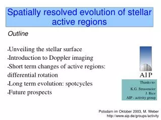
Spatially resolved evolution of stellar active regions. Outline Unveiling the stellar surface Introduction to Doppler imaging Short term changes of active regions: differential rotation Long term evolution: spotcycles Future prospects. Thanks to:

E N D
Spatially resolved evolution of stellar active regions Outline • Unveiling the stellar surface • Introduction to Doppler imaging • Short term changes of active regions: differential rotation • Long term evolution: spotcycles • Future prospects Thanks to: K.G. StrassmeierJ. RiceAIP - activity group Potsdam im Oktober 2003, M. Weber http://www.aip.de/groups/activity
Sunspots & differential rotation • Equator rotates faster than the pole • “Rigidity” changes throughout the solar cycle and between Odd & Even cycles • Equatorial rotation faster in ONSC
Starspots • Stars exhibit periodic light variations (often rotationally modulated) • Activity-related features found in starspots are present in stellar spectra (e.g. CaII H&K) • Chromospheric emission lines very strong in such stars
Direct imaging of starspots • Faint Object Camera of HST • Interferometric techniques • Only very large & very near objects observable 'direct' image of Betelgeuse Gilliland & Dupree 1996, ApJ
Photometric spot models • Positions and sizes of spots are optimized • Several bandpasses (V,R,I,..) are used for inversion • Only simple spot configurations can be retrieved • Some assumptions have to be made e.g. HK Lac: Oláh et al. 1997
Principle of Doppler imaging Missing flux (in case of a dark spot) leaves a characteristc bump in spectral line profile.
Doppler imaging1 • Missing flux from spots produce line profile deformations • 'bumps' move from blue to red wing of the profile due to the 'Doppler' effect. • Position of spots correspond to spot longitudes
Doppler imaging2 • Speed of spots give indication of the latitude (more uncertain than the longitude) • 'bumps' from high latitude spots start out somewhere in the middle of the line wing, low latitude spots at the shoulder
Short term variations: differential rotation • Artificial star (see Rice & Strassmeier 2000) • = -0.05, P 7days • Note the sign convention for (the solar case is positive) • []=degr/day (x 0.202 = µrad/s) • B & C not independent or:
Simulating differential rotation • line profiles corresponding to 2 rotations of the model star • Using seven consecutive line profiles to reconstruct one image • Simulation of a medium-long (7 day) period star (II Peg)
a. Reconstructing differential rotation by cross-correlation • Artifical maps created using =0.05 and P=6.72 days • Shown is original differential rotation, cross correlation measurements, and fit to cross-correlation • Fit coresponds to =0.06 and P=6.6 days • Introduced for AB Dor by Donati & Collier Cameron (1997) • Observations for two consecutive images needed • Spot/active region lifetimes?
b. “Sheared-image method” • Donati et al. 2000 for RX J1508,6-4423 • Using in inversion process • evaluating 2 for different periods and differential rotation values • Darkest value corresponds to best fit • aka “2 Landscape” method • One image is enough • But longer timeline is an advantage as long as it is smaller than the spot lifetimes
c. Direct tracing of spots AB Dor; Collier Cameron et al. 2002Combining LSD and matched-filter analysis=0.0046 (Peq=0.5132 days)
IM Peg • K2III, Vmax=5.8, vsini=27 • 70 nights of observations • 24.65 days rotation period (SB1) • Two consecutive stellar rotations well covered • Anti-solar differential rotation found ( -0.04)
IM Peg, cont’d Doppler images with 24 days time separation
IM Peg, cont’d • Cross correlation of the two average images • Monte-Carlo style calculation of 50 image-pairs & cross-correlations to estimate the error. • Best fit (red line) corresponds to =1/0=0.58/14.39 = -0.04
IM Peg, cont’d • Including in the inversion procedure “sheared image method” • Parameter variation to find the best fit. • Average value for the four calculations =1/0= -0.04 • Variation of both P and : =1/0= -0.02 ±0.01, P= 24.4 ±0.2
IM Peg, cont’d • 2D-cross correlation reveals meridional flows • Sum of horizontal flow yields the differential rotation pattern • meridional flow appears to be pole-wards
More stars • HD 218153 (K0III, V=7.6) • HD 31993 (K2III, V=7.48) • LQ Hya (K0III, V=7.5) • II Peg (K2IV, V=6.9) • HD 208472, IL Hya, HK Lac
HD 218153 • Differential rotation and meridional flow detected • Weber & Strassmeier 2001 • =0.09 to 0.34 (lower/upper limit)
HD 31993 • Differential rotation detected • Strassmeier et al. 2003 • = -0.15
LQ Hya Donati et al. (in press) ; Kovari et al. (submitted) • P=1.59 days, ≤ 0.05
II Peg • P=6.72days • 5 consecutive Doppler images • -0.05
II Peg cont’d • Using in the inversion leads to a non-zero value for some data sets only. • Dataset for one map spans more than one stellar rotation • and period needs to be varied at the same time • P=6.62±0.05 days, = -0.05±0.02 Variation of and Period (“2-Landscape method”)
Long term changes / Activity cycles • Solar 11yr activity cycle • Mt. Wilson survey found many cycles of solar-type stars • Tracing starspots over one activity cycle is a challenging task (not-only observing) time wise
IM Peg / long term • Active longitudes (Berdyugina et al. 2000) • Probable activity cycle of 6.5yrs • Photometric activity cycles are 29.8 and 10.4 years (Ribarik et al 2003)
II Peg / long term • Long-term variations of spots on II Peg (P9.5yr) • Active longitudes and “flip-flop”; 4.65yr halfcycle • Berdyugina et al. 1999
Variable differential rotation? • Donati et al. (in press) • Differential rotation is different for V and I and for different epochs • Compare to yesterday’s talk by Lanza & Rodonò • Is there a link to activity cycles?
Summary • 5 differential rotation measurements • Single star (HD 218153) has >0, other single star <0 • Kitchatinov & Rüdiger 1999: Prot, meridional flow, larger for giants
Outlook • The availability of several robotic telescope facilities will make long-term studies much easier. • In addition, stars not observable (e.g. P=1day) from one spot cat be observed from several facilities concurrently.