Understanding Discretizing and Instance-based Learning
E N D
Presentation Transcript
Labor Data Sorted by wage-increase-first
Discretizing “wage-increase-first” Split after 2: • avg(entropy[4/5,1/5], entropy[6/21, 15/21]) • entropy[4/5,1/5] = -(4/5)*l(4/5)-(1/5)*l(1/5) = 0.5 • entropy[6/21,15/21] = -(6/21)*l(6/21)-(15/21)*l(15/21) = .598 • avg = (5/26)*0.5 + (21/26)* .598 = .579 Split after 3: • avg(entropy[8/9,1/9], entropy[2/17, 15/17]) • entropy[8/9,1/9] = -(8/9)*l(8/9)-(1/9)*l(1/9) = .349 • entropy[2/17,15/17] = -(2/17)*l(2/17)-(15/17)*l(15/17) = .362 • avg = (9/26)* .349 + (17/26)* .362 = .357 Split after 3.5: • avg(entropy[8/12,4/12], entropy[2/14, 12/14]) • entropy[8/12,4/12] = -(8/12)*l(8/12)-(4/12)*l(4/12) = .637 • entropy[2/14,12/14] = -(2/14)*l(2/14)-(12/14)*l(12/14) = .41 • avg = (12/28)* .637 + (14/28)* .41 = .478
Discretizing “wage-increase-first” • Split after 4: • avg(entropy[10/14,4/14], entropy[0/12,12/12]) • entropy[10/14,4/14] = -(10/14)*l(10/14)-(4/14)*l(4/14) = .598 • entropy[0/12,12/12] = -(0/12)*l(0/12)-(12/12)*l(12/12) = 0 • avg = (14/26)*0.598 + (12/26)* 0 = .322 (the smallest) • No Split: • entropy[10/26,16/26] = -(10/26)*l(10/26)-(16/26)*l(16/26) = .666
Discretizing “wage-increase-first” Need to continue in the yellow part
Discretizing “wage-increase-first” Split after 2: • avg(entropy[4/5,1/5], entropy[6/9, 3/9]) • entropy[4/5,1/5] = -(4/5)*l(4/5)-(1/5)*l(1/5) = .5 • entropy[6/9,3/9] = -(6/9)*l(6/9)-(3/9)*l(3/9) = .637 • avg = (5/14)*0.5 + (9/14)* 0.637 = .588 Split after 3: • avg(entropy[8/9,1/9], entropy[2/5, 3/5]) • entropy[8/9,1/9] = -(8/9)*l(8/9)-(1/9)*l(1/9) = .349 • entropy[2/5,3/5] = -(2/5)*l(2/5)-(3/5)*l(3/5) = .673 • avg = (9/14)* .349 + (5/14)* .673 = .465 Split after 3.5: • avg(entropy[8/12,4/12], entropy[2/2, 0/2]) • entropy[8/12,4/12] = -(8/12)*l(8/12)-(4/12)*l(4/12) = .637 • entropy[2/2,0/2] = -(2/2)*l(2/2)-(0/2)*l(0/2) = 0 • avg = (12/14)* .637 + (2/14)* 0 = .546
Discretizing “wage-increase-first” • No Split: • entropy[10/14,4/14] = -(10/14)*l(10/14)-(4/14)*l(4/14) = .598 • So, we need to split “after 3.”
Discretizing “wage-increase-first” Need to continue in the yellow part, as well as in the red part. For the yellow part it’s easy: There is only one choice, which makes the entropy perfect. What about the red part?
Discretizing “wage-increase-first” What about the red part? Should we split further?
Discretizing “wage-increase-first” • Split after 2: • avg(entropy[4/5,1/5], entropy[4/4, 0/4]) • entropy[4/5,1/5] = -(4/5)*l(4/5)-(1/5)*l(1/5) = .5 • entropy[4/4,0/4] = 0 • avg = (5/9)*0.5 + (4/9)* 0 = .278 • No Split: • entropy[8/9,1/9] • entropy[8/9,1/9] = -(8/9)*l(8/9)-(1/9)*l(1/9) = .349 • So, it’s better to split. • You might get the impression that we split after each value. I.e. there would be one discrete value for each numeric value. • However, had we 13 instances in the red part as opposed to 9, there would be no split “after 2” • -(12/13)*l(12/13)-(1/13)*l(1/13) = .271
Instance-based learning: IB2 • IB2: save memory, speed up classification • Work incrementally • Only incorporate misclassified instances • Problem: noisy data gets incorporated Data: “Who buys gold jewelry” (25,60,no) (45,60,no) (50,75,no) (50,100,no) (50,120,no) (70,110,yes) (85,140,yes) (30,260,yes) (25,400,yes) (45,350,yes) (50,275,yes) (60,260,yes)
Instance-based learning: IB2 • Data: • (25,60,no) • (85,140,yes) • (45,60,no) • (30,260,yes) • (50,75,no) • (50,120,no) • (70,110,yes) • (25,400,yes) • (50,100,no) • (45,350,yes) • (50,275,yes) • (60,260,yes) This is the final answer. I.e. we memorize only these 5 points. However, let’s compute gradually the classifier.
Instance-based learning: IB2 • Data: • (25,60,no)
Instance-based learning: IB2 • Data: • (25,60,no) • (85,140,yes) Since so far the model has only the first instance memorized, this second instance gets wrongly classified. So, we memorize it as well.
Instance-based learning: IB2 • Data: • (25,60,no) • (85,140,yes) • (45,60,no) So far the model has the two first instances memorized. The third instance gets properly classified, since it happens to be closer with the first. So, we don’t memorize it.
Instance-based learning: IB2 • Data: • (25,60,no) • (85,140,yes) • (45,60,no) • (30,260,yes) So far the model has the two first instances memorized. The fourth instance gets properly classified, since it happens to be closer with the second. So, we don’t memorize it.
Instance-based learning: IB2 • Data: • (25,60,no) • (85,140,yes) • (45,60,no) • (30,260,yes) • (50,75,no) So far the model has the two first instances memorized. The fifth instance gets properly classified, since it happens to be closer with the first. So, we don’t memorize it.
Instance-based learning: IB2 • Data: • (25,60,no) • (85,140,yes) • (45,60,no) • (30,260,yes) • (50,75,no) • (50,120,no) So far the model has the two first instances memorized. The sixth instance gets wrongly classified, since it happens to be closer with the second. So, we memorize it.
Instance-based learning: IB2 • Continuing in a similar way, we finally get, the figure in the right. • The colored points are the one that get memorized. This is the final answer. I.e. we memorize only these 5 points.
Instance-based learning: IB3 • IB3: deal with noise • Discard instances that don’t perform well • Keep a record of the number of correct and incorrect classification decisions that each exemplar makes. • Two predetermined thresholds are set on success ratio. • An instance is used for training: • If the number of incorrect classifications is the first threshold, and • If the number of correct classifications the second threshold.
Instance-based learning: IB3 • Suppose the lower threshold is 0, and upper threshold is 1. • Shuffle the data first • (25,60,no) • (85,140,yes) • (45,60,no) • (30,260,yes) • (50,75,no) • (50,120,no) • (70,110,yes) • (25,400,yes) • (50,100,no) • (45,350,yes) • (50,275,yes) • (60,260,yes)
Instance-based learning: IB3 • Suppose the lower threshold is 0, and upper threshold is 1. • Shuffle the data first • (25,60,no) [1,1] • (85,140,yes) [1,1] • (45,60,no) [0,1] • (30,260,yes) [0,2] • (50,75,no) [0,1] • (50,120,no) [0,1] • (70,110,yes) [0,0] • (25,400,yes) [0,1] • (50,100,no) [0,0] • (45,350,yes) [0,0] • (50,275,yes) [0,1] • (60,260,yes) [0,0]
Instance-based learning: IB3 • The points that will be used in classification are: • (45,60,no) [0,1] • (30,260,yes) [0,2] • (50,75,no) [0,1] • (50,120,no) [0,1] • (25,400,yes) [0,1] • (50,275,yes) [0,1]
Rectangular generalizations • When a new exemplar is classified correctly, it is generalized by simply merging it with the nearest exemplar. • The nearest exemplar may be either a single instance or a hyper-rectangle.
Rectangular generalizations • Data: • (25,60,no) • (85,140,yes) • (45,60,no) • (30,260,yes) • (50,75,no) • (50,120,no) • (70,110,yes) • (25,400,yes) • (50,100,no) • (45,350,yes) • (50,275,yes) • (60,260,yes)
Classification • If the new instance lies within a rectangle then output the rectangle class • If the new instance lies in the overlap of several rectangles, then output the class of the rectangle whose center is the closest to the new data instance. • If the new instance lies outside any of the rectangles, output the class of the rectangle, which is the closest to the data instance. • The distance of a point from a rectangle is: • If an instance lies within rectangle, d=0 • If outside, d = distance from the closest rectangle part, i.e. distance from some point in the rectangle boundary. Class 1 Class 2 Separation line
Exercise Assuming that the salary is the class attribute • Build a decision tree using ID3 • Build a Naïve Bayes model
