Download
1 / 34
340 likes | 368 Views
Learn about robust estimators and Random Sample Consensus algorithm for segmentation in computer vision. Understand how outliers affect parameter estimation and explore methods to improve model fitting accuracy.

E N D
Segmentation by fitting a model: robust estimators and RANSAC T-11 Computer Vision University of Ioannina Christophoros Nikou Images and slides from: James Hayes, Brown University, Computer Vision course D. Forsyth and J. Ponce. Computer Vision: A Modern Approach, Prentice Hall, 2003. Computer Vision course by Svetlana Lazebnik, University of North Carolina at Chapel Hill. Computer Vision course by Kristen Grauman, University of Texas at Austin.
Least squares and outliers Problem: squared error heavily penalizes outliers.
Least squares and outliers The y-coordinate of a point corrupted. The error seems small…
Least squares and outliers Zoom into the previous example to highlight the error.
Robust estimators • In the least squares case, we minimize the residual r(xi, θ) with respect to the model parameters θ: • Outliers contribute too much to the estimation of the parameters θ. • A solution is to replace the square with another function less influenced by outliers. • This function should behave like the square for “good” points.
Robust estimators The robust function ρ behaves like a squared distance for small values of its argument but saturates for larger values of it. Notice the role of parameter σ. We have to select it carefully.
Robust estimators • Estimation of the model parameters is now obtained by: where ψ(x;σ)is the influence function of the robust estimator characterizing the influence of the residuals to the solution.
Robust estimators Standard least squares estimator and its influence function
Robust estimators Truncated least squares estimator and its influence function
Robust estimators Geman-McClure estimator and its influence function
Robust estimators Correct selection of σ: the effect of the outlier is eliminated
Robust estimators Small σ: the error value is almost the same for every point and the fit is very poor. All the points are considered as outliers.
Robust estimators Large σ: the error value is like least squares and the fit is very poor. All the points are considered as “good”.
Robust estimation • Robust fitting is a nonlinear optimization problem that must be solved iteratively. • Least squares solution can be used for initialization. • Adaptive choice of scale base on the median absolute deviation (MAD) of the residuals at each iteration (t): • It is based on the MAD of normally distributed points with standard deviation of 1. P. Rousseeuw and A. Leory. Robust regression and outlier detection. J. Wiley 1987.
RANSAC • Robust fitting can deal with a few outliers – what if we have many of them? • Random sample consensus (RANSAC) • Choose a small subset of points uniformly at random. • Fit a model to that subset. • Find all remaining points that are “close” to the model and reject the rest as outliers. • Do this many times and choose the best model. M. A. Fischler and R. C. Bolles. Random Sample Consensus: A Paradigm for Model Fitting with Applications to Image Analysis and Automated Cartography. Communications of the ACM, Vol 24, pp 381-395, 1981.
RANSAC • Insight • Search for “good”: points in the data set. • Suppose we want to fit a line to a point set degraded by at 50% by outliers. • Choosing randomly 2 points has a chance of 0.25 to obtain “good” points. • We can identify them by noticing that a many other points will be close to the line fitted to the pair. • Then we fit a line to all these “good” points. M. A. Fischler and R. C. Bolles. Random Sample Consensus: A Paradigm for Model Fitting with Applications to Image Analysis and Automated Cartography. Communications of the ACM, Vol 24, pp 381-395, 1981.
RANSAC (RANdom SAmple Consensus) : Fischler & Bolles in ‘81. Algorithm: • Sample (randomly) the number of points required to fit the model • Solve for model parameters using samples • Score by the fraction of inliers within a preset threshold of the model Repeat 1-3 until the best model is found with high confidence
RANSAC Line fitting example Algorithm: • Sample (randomly) the number of points required to fit the model (n=2) • Solve for model parameters using samples • Score by the fraction of inliers within a preset threshold of the model Repeat 1-3 until the best model is found with high confidence Illustration by Savarese
RANSAC Line fitting example Algorithm: • Sample (randomly) the number of points required to fit the model (n=2) • Solve for model parameters using samples • Score by the fraction of inliers within a preset threshold of the model Repeat 1-3 until the best model is found with high confidence
RANSAC Line fitting example Algorithm: • Sample (randomly) the number of points required to fit the model (#=2) • Solve for model parameters using samples • Score by the fraction of inliers within a preset threshold of the model Repeat 1-3 until the best model is found with high confidence
RANSAC Algorithm: • Sample (randomly) the number of points required to fit the model (n=2) • Solve for model parameters using samples • Score by the fraction of inliers within a preset threshold of the model Repeat 1-3 until the best model is found with high confidence
RANSAC • Repeat k times: • Draw n points uniformly at random. • Fit line to these n points. • Find inliers to this line among the remaining points (i.e., points whose distance from the line is less than t). • If there are d or more inliers, accept the line (and the consensus set) and refit to all inliers. • Select the largest consensus set. Parameters k, n, t and d are crucial.
RANSAC • Number of samples n and number of iterations k. • The minimum number to fit the model (2 points for lines). • If w is the fraction of “good” points, the expected number of draws required to get a “good” sample is: E[k]=1 x p(one good sample in one draw) + 2 x p(one good sample in two draws) + … = wn +2(1-wn) wn+3(1-wn)2wn+…= w-n. We add a few standard deviations to this number:
RANSAC • Number of iterations k (alternative approach). • We look for a number of samples that guarantees a that at least one of them is free from outliers with a probability of p. • Probability of seeing a bad sample of points in one draw: • and the probability of seeing only bad samples in k draws is: Solving for k:
RANSAC • The number of iterations k required to ensure, with a probability p=0.99, that at least one sample has no outliers for a given size of sample, n, and proportion of outliers 1-w.
RANSAC • Threshold t to decide if a point is close to the line or not. • We generally specify it as a part of the modeling process. • The same as in the maximum likelihood formulation of line fitting (parameter σ). • Look similar data sets, fit some lines by eye and determine it empirically.
RANSAC • Number of points d that must be close to the line (the size of the consensus set). • A rule of thumb is to terminate if the size of the consensus set is similar to the number of inliers believed to be in the data set, given the assumed proportion of outliers. • For N data points and if the percentage of inliers is w:
RANSAC • Pros • Simple and general. • Applicable to many different problems. • Often works well in practice. • Cons • Lots of parameters to tune. • Can’t always get a good initialization of the model based on the minimum number of samples. • Sometimes too many iterations are required. • Can fail for extremely low inlier ratios. • We can often do better than brute-force sampling.
Fitting using probabilistic methods • Straightforward to build probabilistic models. • Generative model for the data. • Simple line fitting: the same equations as least squares arise. • The x coordinate is uniformly distributed. • The y coordinate is ax+b plus Gaussian noise. • Estimate the parameters of the straight line by maximizing the likelihood of the data points.
Fitting using probabilistic methods • Maximum likelihood (ML) • We usually minimize the negative log-likelihood • Setting the derivatives w.r.t. the parameters equal to zero yields the least squares solution.
Fitting using probabilistic methods • Total least squares fitting with ML • a point (u,v) on the line is generated by a uniform pdf. • a distance ξis sampled form a Gaussian pdf to perturbate the original point along a direction perpendicular to the line. • If the line is ax+by+c=0, then
Fitting using probabilistic methods ax+by+c=0 • Generative model: line points are corrupted by Gaussian noise in the direction perpendicular to the line (u, v) ε (x, y) point on the line noise:zero-meanGaussian withstd. dev. σ normaldirection
Fitting using probabilistic methods • For fixed, but unknown σ,this yields the problem we were working in the previous section.