Measuring and Modeling Hyper-threaded Processor Performance
Measuring and Modeling Hyper-threaded Processor Performance. Ethan Bolker UMass-Boston September 17, 2003. Joint work with Yiping Ding, Arjun Kumar (BMC Software) Accepted for presentation at CMG32, December 2003 Paper (with references) available on request. Improving Processor Performance.

Measuring and Modeling Hyper-threaded Processor Performance
E N D
Presentation Transcript
Measuring and Modeling Hyper-threaded Processor Performance Ethan Bolker UMass-Boston September 17, 2003
Joint work with Yiping Ding, Arjun Kumar (BMC Software) • Accepted for presentation at CMG32, December 2003 • Paper (with references) available on request
Improving Processor Performance • Speed up clock • Invent revolutionary new architecture • Replicate processors (parallel application) • Remove bottlenecks (use idle ALU) • caches • pipelining • prefetch
Hyper-threading Technology (HTT)Default for new Intel high end chips • One ALU • Duplicate state of computation (registers) to create two logical processors (chip size *= 1.05) • Parallel instruction preparation (decode) • ALU should see ready work more often (provided there are two active threads)
The path to instruction execution Intel Technology Journal, Volume 06 Issue 01, February 14, 2002, p8
How little must we understand? • Batch workload: repeated dispatch of identical compute intensive jobs • vary number of threads • measure throughput (jobs/second) • Treat processor as a black box • Experiment to observe behavior • Model to predict behavior
} puzzling } makes sense } make sense Batch throughput
Transaction processing • More interesting than batch • Random size jobs arrive at random times • M/M/1 M = “Markov” M/*/*: arrival stream is Poisson, rate */M/*: job size exponentially distributed, mean s */*/1: single processor
M/M/1 model evaluation • Utilization: U = s U is dimensionless: jobs/sec * sec/job U < 1 else saturation • Response time: r = s/(1-U) randomness each job sees (virtual) processor slowed down (by other jobs) by factor 1/(1-U), so to accumulate s seconds of real work takes r = s/(1-U) seconds of real time
Benchmark • Java driver • chooses interarrival times and service times from exponential distributions, • dispatches each job in its own thread, • records actual job CPU usage, response time • Input parameters • job arrival rate • mean job service time s • Fix s = 1 second, vary (hence U), track r
practice: measured theory: M/M/1 R = 1/(1-U) Benchmark validation
Theory vs practice • “In theory, there is no difference between theory and practice. In practice, there is no relationship between theory and practice.” Grant Gainey • “The gap between theory and practice in practice is much larger than the gap between theory and practice in theory.” Jeff Case
Explain/remove discrepancy • Examine, tune benchmark driver • Compute actual coefficients of variation, incorporate in corrected M/M/1 formula • Nothing helps • Postpone worry – in the meanwhile …
HTT on vs HTT off • Use this benchmark to measure the effect of hyper-threading on response time • Use throughput () as the independent variable • “Utilization” is ambiguous (digression)
What’s happening • Hyper-threading allows more of the application parallelism to make its way to the ALU • Can we understand this quantitatively?
preparatory phase service time s1 execution phase service time s2 /2 /2 s1 s2 r = + 1 – (/2) s1 1 – s2 Model HTT architecture
Theory vs practice s1 = 0.13 s2 = 0.81
Model parameters • To compute response time r from model, need (virtual) service parameters s1, s2( is known) • Finding s1, s2 • eyeball measured data • fit two data points • maximum likelihood • derive from first principles • s1 = 0.13, s2 = 0.81 make sense 15% of work is preparatory, 85% execution
Benchmark validation (reprise) • Chip hardware unchanged when HTT off • Assume one path used • Tandem queue • Parameter estimation as before 0
Theory vs practice s1 = 0.045 s2 = 0.878
Future work • Do serious statistics • Does 1+1 tandem queue model predict hyper-threading response as well as complex 2+1 model? • Understand two-processor machine puzzle • Explore how s1 and s2 vary with application (e.g. fixed vs floating point) • Find ways to estimate s1 and s2 from first principles
Summary • Hyper-threading is … • Abstraction (modelling) leverages information: you can often understand a lot even when you know very little • r = s/(1-U) is worth remembering • You do need to connect theory and practice – and practice is harder than theory • Questions?