MODEL SIMULATIONS

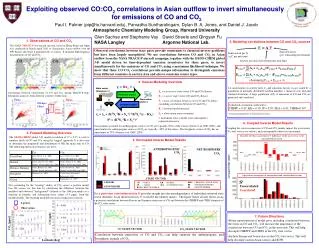
1. Japan China Slope (> 840 mb) = 22 R2 = 0.45 Slope (> 840 mb) = 51 R2 = 0.76 Offshore China Over Japan Glen Sachse and Stephanie Vay NASA Langley David Streets and Qingyan Fu Argonne National Lab. (Assuming FCO + FCO2 = 1) y = Kxa +  State vector (Emissions x) Forward model Observation vector y Inverse model 6. Coupled Inverse Model Results Coupling the errors in emissions of CO and CO2 mainly impact the a posteriori CO2 state vector (see below), and consequently reduces its uncertainty. xs = xa + (KTSy-1K + Sa-1)-1 KTSy-1(y – Kxa) SS = (KTSy-1K + Sa-1)-1 Absolute (red bars) and relative % difference of the state vector to the uncorrelated inversion 6.7% 7.0.% 0.9% 0.1% 11.4% 0.1% 5.5% 0.0% -1.9% -2.0% -9.4% -5.0% -5.8% -43.7% -11.4% (see panel 4 for units) -9.7% A posteriori uncertainty of uncorrelated and correlated inversions Ss Uncorrelated Correlated BFFF = BIOFUEL + FOSSIL FUEL BB = BIOMASS BURNING BS = NET BIOSPHERE CH = CHINA KR = KOREA JP = JAPAN SEA = SOUTHEAST ASIA ROW = REST OF WORLD ECO = (Ai + A,iA,i)(1 – (FCO2,I+F,CO2,iCO2,i)) A priori Sector i Observation ECO2 = (Ai + A,iA,i)(FCO2,i + F,CO2,iCO2,I ) Sector i CO2 [ppm] MODEL SIMULATIONS Exploiting observed CO:CO2 correlations in Asian outflow to invert simultaneously for emissions of CO and CO2 Paul I. Palmer (pip@io.harvard.edu), Parvadha Suntharalingam, Dylan B. A. Jones, and Daniel J. Jacob Atmospheric Chemistry Modeling Group, Harvard University 1. Observations of CO and CO2 5. Modeling correlations between CO and CO2 sources The NASATRACE-Ptwo-aircraft mission, based in Hong Kong and Japan, was conducted in March-April 2001 to characterize Asian outflow over the NW Pacific and relate it quantitatively to sources. It included high-frequency measurements of CO and CO2: E = AF Observed correlations between trace gases provide constraints to chemical inverse problems but have been largely unexploited. We use correlations between CO and CO2 in Asian outflow from the NASA TRACE-P aircraft campaign, together with the GEOS-CHEM global 3-D model driven by time-dependent emission inventories for these gases, to invert simultaneously for the emissions of CO and CO2 using a maximum likelihood technique. We show that these CO:CO2 correlations provide unique information to distinguish emissions from different countries in eastern Asia and also to constrain source types. Emission factor (g C released/kg fuel burned) Emission of gas X (g C per unit time) CO CO2 Activity rate (kg of fuel burned per unit time) 3. Inverse Modeling Overview 1- uncertainties in activity rates A and emissions factors F are scaled by a population of normally distributed random numbers  (mean of zero and unit standard deviation). A large population (104) of emissions of CO and CO2 are generated and correlated. Xs= a posteriori state vector (CO and CO2 fluxes) Xa= a priori state vector (CO and CO2 fluxes) Sa= error covariance of the a priori CO and CO2 fluxes (including correlations between CO and CO2) K = forward model operator Sy = observation error covariance = instrument error + model error (uncoupled) + representation error Correlations between observations of CO and CO2 during TRACE-P help distinguish airmasses from different countries within Asia: Japan China Offshore China Calculated correlation coefficients r: CHBFF = 0.47; KR = 0.39; JP = 0.39; SEA = 0.41; CHBB=0.30* Over Japan * Estimated independently of method described above MODEL SIMULATIONS Uncertainties assumed for anthropogenic sources of CO are typically >50% of the source (Streets et al, JGR, 2003); and uncertainties for anthropogenic sources of CO2 are typically ~20% of the source. The biospheric source of CO2 has an uncertainty of 75% (Gurney et al, GBC, 2003). 2. Forward Modeling Overview The GEOS-CHEM global 3-D model (resolution of 2o x 2.5o) is used to simulate fields of CO and CO2 using the ‘tagged’ approach. It is also used to determine the magnitude and distribution of OH, the main sink of CO. The following emission inventories are used: 4. Uncoupled Inverse Model Results ANTHROPOGENIC NET BIOSPHERE CO CO2 CO2 STATE VECTOR A PRIORI A POSTERIORI Not accounting for the “missing” sink(s) of CO2 causes a positive model bias We correct for this bias by calculating the difference between the modeled and observed “background” (defined as the 10th percentile) as a function of latitude, and subtracting these values (4-5 ppm), from the modeled fields. The resulting model/observation comparison is shown: The a posteriori correlation matrix Ssprovides insight into the interdependency of individual retrieved state vector elements. In an ideal inversion, Ss would be the identity matrix. The figure below clearly shows strong a posteriori correlations between Korean and Japanese emissions of CO and between the CHBFFF and CHBS elements of the CO2 state vector. 7. Future Directions CO [ppb] • Better representation of model error, including correlations between the errors in CO and CO2, will increase the importance of the correlations between CO and CO2 in the inversion. This will help decouple CHBFFF and CHBS in the CO2 state vector. • Include Europe and boreal Asia in the CO2 state vector. This will help decouple eastern Asian sources and ROW. CO STATE VECTOR CO2 STATE VECTOR Correlation between emissions of CO and CO2 can help separate the anthropogenic and biospheric signals of CO2. Latitude [deg]