Probability theory Random variables
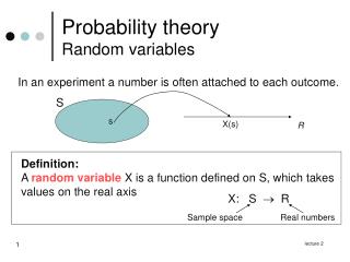
Probability theory Random variables. In an experiment a number is often attached to each outcome. S. s. X(s). R. Definition: A random variable X is a function defined on S, which takes values on the real axis. X: S R. Sample space. Real numbers.

Probability theory Random variables
E N D
Presentation Transcript
Probability theoryRandom variables In an experiment a number is often attached to each outcome. S s X(s) R Definition: A random variableX is a function defined on S, which takes values on the real axis X: S R Sample space Real numbers lecture 2
Probability theoryRandom variables Example: Random variable Type Number of eyes when rolling a dice discrete The sum of eyes when rolling two dice discrete Number of children in a family discrete Age of first-time mother discrete Time of running 5 km continuous Amount of sugar in a coke continuous Height of males continuous counting measure Discrete: can take a finite number of values or an infinite but countable number of values. Continuous: takes values from the set of real numbers. lecture 2
Discrete random variableProbability function • Definition: • Let X : S R be a discrete random variable. • The function f(x) is a probabilty function for X, if • 1. f(x) 0 for all x • 2. • 3. P(X = x) = f(x), • where P(X=x) is the probability for the outcomes sS : X(s) = x. lecture 2
Discrete random variableProbability function Example: Flip three coins X : # heads X : S {0,1,2,3} Value of X X=0 X=1 X=2 X=3 Probability fuinction f(0) = P(X=0) = 1/8 f(1) = P(X=1) = 3/8 f(2) = P(X=2) = 3/8 f(3) = P(X=3) = 1/8 Outcome TTT HTT, TTH, THT HHT, HTH, THH HHH • Notice!The definition of a probability function is fulfilled: • 1. f(x) 0 • 2. f(x) = 1 • 3. P(X=x) = f(x) lecture 2
Discrete random variableCumulative distribution function • Definition: • Let X : S R be a discrete random variable with probability function f(x). • The cumulative distribution function for X, F(x), is defined by • F(x) = P(X x) = for - < x < lecture 2
Discrete random variableCumulative distribution function Example: Flip three coins X : # heads X : S {0,1,2,3} Outcome TTT HTT, TTH, THT HHT, HTH, THH HHH Value of X X=0 X=1 X=2 X=3 Probability function f(0) = P(X=0) = 1/8 f(1) = P(X=1) = 3/8 f(2) = P(X=2) = 3/8 f(3) = P(X=3) = 1/8 Cumulative dist. Func. F(0) = P(X < 0) = 1/8 F(1) = P(X < 1) = 4/8 F(2) = P(X < 2) = 7/8 F(3) = P(X < 3) = 1 Probability function: Cumulative distribution function: F(x) 1.0 f(x) 0.4 0.8 0.3 0.6 0.2 0.4 0.1 0.2 x 0 1 2 3 x 0 1 2 3 lecture 2
Continuous random variable • A continuous random variable X has probability 0 for all outcomes!! • Mathematically: P(X = x) = f(x) = 0 for all x Hence, we cannot represent the probability function f(x) by a table or bar chart as in the case of discrtete random variabes. Instead we use a continuous function – a density function. lecture 2
Continuous random variableDensity function • Definition: • Let X: S R be a continuous random variables. • A probability density functionf(x) for X is defined by: • 1. f(x) 0 for all x • 2. • 3. P( a < X < b ) = f(x) dx • Note!!Continuity: P(a < X < b) = P(a < X < b) = P(a < X < b) = P(a < X < b) b a lecture 2
Continuous random variableDensity function Example: X: service life of car battery in years (contiuous) Density function: 3 • Probability of a service life longer than 3 years: lecture 2
Continuous random variableDensity function Alternativ måde: 3 • Probability of a service life longer than 3 years: lecture 2
Continuous random variableDensity function • Definition: • Let X : S R be a contiguous random variable with density function f(x). • The cumulative distribution function for X, F(x), er defined by • F(x) = P(X x) = for - < x < • Note: F´(x) = f(x) 3 lecture 2
Continuous random variableDensity function From the definition of the cumulative distribution funct. we get: P( a < X < b ) = P( a < X < b ) = P( a < X < b ) = P( a < X < b ) = P(X < b ) – P(X < a ) = F(b) – F(a) a b lecture 2
Continuous random variableDensity function • Discrete random variable • Sample space is finite or has countable many outcomes • Probability function f(x) • Is often given by table • Calculation of probabilities • P( a < X < b) = f(t) • Contiuous random variable • The sample space contains infinitely many outcomes • Density function f(x) is a • Continuous function • Calculation of probabilities • P( a < X < b ) = f(t) dt b a a<t<b lecture 2
Joint distribution Joint probability function • Definition: • Let X and Y be two discrete random variables. • The joint probability function f(x,y) for X and Y • Is defined by • 1. f(x,y) 0 for all x og y • 2. • 3. P(X = x ,Y = y) = f(x,y) (the probability that both X = x and Y=y) • For a set A in the xy plane: lecture 2
Joint distribution Marginal probability function • Definition: • Let X and Y be two discrete random variables with joint probability function f(x,y). • The marginal probability function for X is given by • g(x) = f(x,y) for all x • The marginal probability function for Y is given by • h(y) = f(x,y) for all y y x lecture 2
Joint distribution Marginal probability function Example 3.14 (modified): The joint probability function f(x,y) for X and Y is given by x 0 1 2 0 3/28 3/14 1/28 1 9/28 3/14 0 2 3/28 0 0 y • h(1) = P(Y =1) = 3/14+3/14+0 = 3/7 • g(2) = P(X= 2) = 3/28+0+0 = 3/28 • P(X+Y < 2) = 3/28+9/28+3/14 = 18/28 = 9/14 lecture 2
Joint distributionJoint density function • Definition: • Let X og Y be two continuous random variables. • The joint density function f(x,y) for X and Y is • defined by • 1. f(x,y) 0 for all x • 2. • 3. P(a < X< b, c<Y< d) = • For a region A in the xy-plane: P[(X,Y)A] = f(x,y) dxdy A lecture 2
Joint distributionMarginal density function • Definition: • Let X and Y be two continuous random variables with joint density function f(x,y). • The marginal density functionfor X is given by • The marginal density functionfor Y is given by lecture 2
Joint distributionMarginal density function • Example 3.15 + 3.17 (modified): • Joint density f(x,y) for X and Y: • Marginal density function for X: lecture 2
Joint distributionConditional density and probability functions Definition: Let X and Y be random variables (continuous or discrete) with joint density/probability function f(x,y). Then the Conditional denisty/probability functionfor Y given X=x is f(y|x) = f(x,y) / g(x) g(x) 0 where g(x) is the marginal density/probability function for X, and the conditional density/probability function for X given Y=y is f(x|y) = f(x,y) / h(y) h(y) 0 where h(y) is the marginal density/probability function for Y. lecture 2
Joint distributionConditional probability function Examples 3.16 + 3.18 (modified): Joint probability function f(x,y) for X and Y is given by: • marginal pf. • P(Y=1 | X=1 ) = f(1|1) • = f(1,1) / g(1) • = (3/14) / (15/28) • = 6/15 x 0 1 2 1 9/28 3/14 0 0 3/28 3/14 1/28 2 3/28 0 0 y lecture 2
Joint distributionIndependence Definition: Two random variables X and Y (continuous or discrete) with joint density/probability functions f(x,y) and marginal density/probability functions g(x) and h(y), respectively, are said to be independent if and only if f(x,y) = g(x) h(y) for all x,y or if f(x|y) = g(x) (x indep. of y) or f(y|x)=h(y) (y indep. af x) lecture 2