Global Climate Change - Evidence and Effects One of the concerns facing humanity is our effect on climates, due largely

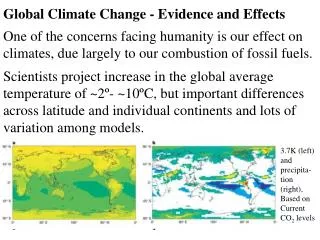
1. Global Climate Change - Evidence and Effects One of the concerns facing humanity is our effect on climates, due largely to our combustion of fossil fuels. Scientists project increase in the global average temperature of ~2º- ~10ºC, but important differences across latitude and individual continents and lots of variation among models. 3.7K (left) and precipita-tion (right), Based on Current CO2 levels

2. 10.5K and predipitationbased on a doubling of CO2 Why do they project increased temperature? Is there historical evidence that leads to these projections? How do projections differ among latitudinal zones? If the projections are accurate, the effects on species diversity, the patterns of species' distributions, agricultural production, and sea level will by vast. The Evidence:

3. 1. The Historical Evidence – Gases trapped in glacial ice tell us what atmospheres were like in the past. Cores have been taken on Greenland and in the Antarctic. The Vostok core (Russian Antarcitica) is the major source for this figure… Wisconsin glaciation

4. We have various sources to estimate climate over a much longer span, at least 55-60 MY. During Pleistocene glaciation, temperatures were cooler than today, but this figure does not show recent warming very well.

5. More recent increases in CO2 are better documented with data from the Mauna Loa observatory in Hawaii, well isolated from major industrial sources, and therefore a good indicator of global pattern.

6. If we look at data from Mauna Loa in greater detail, the seasonal cycle is evident. In winter in the northern hemisphere, photosynthesis is reduced, but not atmospheric input of CO2.

7. Recent increase looks approximately exponential. Global climate and CO2 have changed in the past naturally. How do we know we are responsible for the recent increase? 1) The exponential increase over the last 150 years has three "breaks". Those breaks match with the First and Second World Wars and the Great Depression. They are the three breaks in global economic activity. 2) Isotopic ratios between C12 and C14 indicate fossil fuel combustion is the source of increasing CO2 concentration.

8. The half life of C14 is 5,730 years. It decays into N14 by conversion of a neutron into a proton. C14 is formed by the reverse conversion in the atmosphere when a thermal neutron displaces a proton as a result of cosmic radiation in the upper atmosphere. The rate of C14 formation is essentially constant. Living plants and animals take up C14 and C12 with little selectivity (though there is selectivity against C13, particularly in C3 plants). Fossil fuels were formed millions of years ago. C14 in them will have decayed after hundreds of half-lives. What we find is an enormous depletion of C14 relative to C12 in fuels compared to living plants.

9. If increasing carbon dioxide in the atmosphere is due to fossil fuel combustion, rather than some sort of natural change in current source-sink relationships, then the isotopic ratio should have changed over time due to the release of carbon with an enormously reduced C14 content. The reduced ratio is called the Suess effect. It is clearly evident. from Baxter and Walton (1970)

11. What are the predicted biological impacts of the changes associated with global warming, and are some of these changes already apparent? Hughes (2000) argued that changes are evident, and presented some of the patterns evident and expected from global warming.

12. Plant growth physiology changes in increased CO2 atmospheres. Generally, growth rates increase, and warming lengthens the growing season for plants. The density of stomates decreases in many species, since fewer openings are necessary to take in sufficient CO2. • 2. Species distributions change. Population sizes of • native vascular plants on Antarctica have increased • dramatically (by ~25x) from 1964-1990. Treelines • have moved upward along mountain slopes since • the turn of the 20th century. The ranges of non- • migratory European butterflies have generally • shifted northward by 35-240 kilometers (22 of 35 • species, only 2 shifted southward).

13. 3. The malaria plasmodium and its mosquito vector now occur at higher elevations in Asia, Central America, and Latin America. Dengue fever, previously limited to 1000m elevation, reached 1700m in Mexico and 2200m in Colombia. 4. Birds have similarly extended their distributions northward. In Britain, 59 bird species from the southern portion had extended distributions northward by an average of 19 km over 20 years (1968-72 compared with 1988-91).

14. 5. Life cycles and the timing of critical seasonal events have changed. Egg laying in insects and birds, flowering and seed set in plants typically occur days earlier. Development may occur more rapidly, particularly in insects. Initial flight in holometabolous species (e.g. Lepidoptera) may occur earlier. Let’s look at some of these changes and their impacts on conservation in greater detail.

15. Just in case you think all the global warming evidence suggests uniform warming and changes that might lead to to expect, we’ll first consider the sea ice conditions in the regions where narwhals overwinter. The predictions are that arctic ice will be reduced in extent and thickness on average, opening sea lanes above Canada and Russia. That has not been the case in the wintering grounds of the narwhal in Baffin Bay (Laidre and Heide-Jorgenson, 2005). Instead, the amount of open water required for narwhal to breathe has been declining in recent decades.

16. March sea ice in Baffin Bay – NWG is the narwhal’s northern wintering ground, and SWG the southern wintering ground. How has the extent of sea ice changed over recent decades? Fraction of open water variability

17. Narwhal arrive at the wintering grounds when there is around 60% open water. Then freeze up limits their movements. They nevertheless show great site fidelity. Increasing sea ice in the wintering grounds probably affects their feeding. They cannot move away from open leads where they breathe. Increasing sea ice, increased Greenlandic fishing for their main winter food (Greenland halibut), and Inuit hunting all increase the species’ vulnerability. There is genetic evidence (one of the lowest measures of genetic diversity of all marine mammals) that the narwhal went through an earlier bottleneck, but survived.

18. Climate change, as it occurs, will alter ocean temperatures, currents, ice formation, and sea level. These changes will affect a broad variety of sea mammals, not just narwhal. Cetaceans will be among the most vulnerable and likely to be negatively affected. Cetaceans would be affected by changes in their prey both in terms of productivity and shifts in distribution of prey species. • Five other related issues: • The rate of climate change is outside the evolutionary experience of existing cetacean species.

19. (2) Many whale species have complicated life cycles and appear to be dependent on finding certain resources in certain places at certain times. (3) Movement of water bodies and changes in temperature could affect the ability of whales to navigate across the oceans. (4) Many whale populations are already at extremely low levels. (5) Species and populations are concurrently being negatively affected by other factors.

20. Here’s a table of marine mammals and their conservation status (from Simmonds and Isaac 2007):

21. What will the effects on marine mammals be? Colder water species will shift towards the poles and, ultimately, this will probably result in a reduced global range for these species. Some of this is response to changes in prey distribution. Example: Cetacean relative abundance in north-west Scotland suggested a range expansion of common dolphins Delphinus delphis (a warmer water species) and a decrease in range of white-beaked dolphins Lagenorhynchus albirostris.

22. It is not only the large mammal species that will be affected. Melting has increased the input of fresh water into many areas of the North Atlantic (Greene et al. 2008). That change in salinity in coastal shelf regions is affecting abundances and seasonal cycles of phytoplankton, zooplankton, and higher trophic-level consumer populations. There are also a renewed, ongoing series of biogeographic range expansions by boreal plankton, including renewal of the trans-Arctic exchanges of Pacific species with the Atlantic, e.g. the North Pacific diatom species Neodenticula seminae.

23. Application of Predicted Climate to Specific Examples • Mammals on Mountaintops (and associated • communities) • Loss of diversity of boreal small mammals from montane forests of the isolated mountain ranges in the Great Basin of the western is predicted in the U.S. (Brown 1995, 1998). A model of the loss was developed based on a doubling of CO2 and a 3o rise in average temperature. Boreal woodland will move up the mountain by 500m. That significantly decreases the habitat area available to the small mammals.

25. Using species-area relationships for these species that Brown had determined earlier, he was able to predict species losses on each of 19 mountain ranges.

26. Brown went on to predict exactly which small mammals would disappear from which mountains…

27. Common names for species in the previous table Eutamias – chipmunk Neotoma – packrat Spermophilus – ground squirrel Microtus – vole Silvilagus – cottontail rabbit Marmota – marmot Sorex – shrew Mustella – weasel (this one is the ermine) Ochotona – pika Zapus – jumping mouse Lepus - hare

28. 2) Range shifts in temperate, deciduous trees of the Great Lakes region Zapinski and Davis (1989, described in Brown 1998) determined that a number of Great Lakes area tree species had northern limits corresponding to the -15ºC January isotherm. They used the last post-glacial period to estimate the rate at which tree species could migrate, using an artificially high estimate of 100 km/century. Distributions on the next slide show the current distribution on the left, predicted distribution for the end of this century on the right. The gray area indicates the long-term potential distribution given sufficient time for dispersal into new areas.

30. 3) Range shifts in European butterflies and Monarch Butterflies Parmesan et al. studied ranges of non-migratory butterflies over the last century in Europe (Parmesan, et al. 1999). Each species had the northern limit of its range in northern Europe, and the southern limit in southern Europe or northern Africa. Data forced them to study northern and southern limits separately. Northern boundaries moved northward in 65% of 52 species, remained stable in 34%, and moved southward in one species (2%). This is a highly significant result (P << 0.001).

31. Southern boundaries retracted northwards in 22% of 40 species, remained stable for most (72%) and moved southward for two species (5%). This is not a significant northward movement. Changes in northern and southern boundaries could be evaluated together for 35 species. Of these, 63% shifted northwards, 29% were stable at both boundaries, 6% shifted southwards, and 3% extended range both northward and southward. This is a highly significant result. The distance these species moved northward ranged from 35-240 km. Annual mean temperatures have warmed by about 0.8° C during the 20th century.

32. Does this mean that species can adapt to climate change? Yes and no. When climate changes slowly enough, many species can keep up. However, the projected change in temperature during the 21st century is far larger, estimated as 2.1 – 4.6C.

33. 4) Thermal stress in Intertidal Marine Species Helmuth et al. (2002) suggests intertidal species like mussels that live in intertidal areas must be able to withstand aerial exposure during low tides, potentially placing these organisms in thermal stress. The intertidal mussel Mytilus californianus is found along a latitudinal gradient from California to Washington. Study showed that midday exposure of mussels to high temperature will be greater at higher latitudes than at lower ones, in part because variation in tide height will be more pronounced at the higher latitudes.

34. Moreover, areas that sustain higher water temperatures may also experience higher feeding rates by predators (sea stars) whose metabolic activity is positively linked to water temperature.

35. 5) Pending Global extinctions associated with climate change What is expected to happen to biodiversity between now and 2050 if the world warms according to reasonable projections? If we assume that climate warming will reduce suitable habitat areas, then Thomas et al. (2004) determined average extinction risk probabilities for 3 warming scenarios: 0.8 to 1.7° increase: 18% species loss 1.8 to 2.0° increase: 24% species loss >2.0° increase: 35% species loss

36. References and Readings: Baxter, M.S. and A.Walton. 1970. A theoretical approach to the Suess effect. Proc.Roy.Soc. London A 318:213-230. Brown, J.H. 1995. Macroecology. Univ. Chicago Press, Chicago, Ill. Brown, J.H. and M.V. Lomolino. 1998. Biogeography 2nd ed. Sinauer, Sunderland, MA. P.567-9, 601-12. Greene, C.H., A.J. Pershing, T.M. Cronin and N. Ceci. 2008. Arctic climate change and its impacts on the ecology of the North Atlantic. Ecology 89:S24-38. Helmuth, B., C. Harley, P. Halpin, M. O’Donnell, G. Hofmann, and C. Blanchette. 2002. Climate change and latitudinal patterns of intertidal thermal stress. Science 298: 1015-1017. Hughes, L. 2000. Biological consequences of global warming: is the signal already apparent? TREE 15:56-61. Laidre, K.L. and M.P. Heide-Jorgenson. 2005. Arctic sea ice trends and narwhal vulnerabiulity. Biol.Conserv. 121:509-517. Lorius, C., J. Jouzel, C. Ritz, L. Merlivat, N.I. Barkov, Y.S. Korotkevich and V.M. Kotlyakov. 1985. A 150,000-year climatic record from Antarctic ice. Nature 316:591-96.

37. Oberhauser, K. and T. Peterson. 2003. Modeling current and future potential wintering distributions of eastern North American monarch butterflies. Proc. Nat. Acad. Sci. (USA): 100: 14063-14068. Parmesan, C. and G. Yohe. 2003. A globally coherent fingerprint of climate change impacts across natural systems. Nature 421:37-42. Parmesan, C. et al. 1999. Poleward shifts in geographical ranges of butterfly species associated with regional warming. Nature 399:579-583. Root, T.L. et al. 2003. Fingerprints of global warming on wild animals and plants. Nature 421:57-60. Stainforth, D.A. et al. 2005. Uncertainty in predictions of climate response to rising levels of greenhouse gases. Nature 433:403-406. Thomas, C.D. et al. 2004. Extinction risk from climate change. Nature 427: 145-148. Zabinski, C. and M.B. Davis. 1989. Hard times ahead for Great Lakes forests: A climate threshold model predicts responses to CO2-induced climate change. In J.B. Smith and D. Tirpak, eds. The Potential Effects of Global Climate Change on the United States. Appendix D, U.S. E.P.A. Washington, D.C.