Download
1 / 56
570 likes | 722 Views
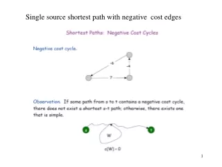
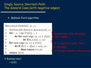
Bellman-Ford algorithm. Iteratively relax all edges |V|-1 times. Single Source Shortest-Path: The General Case (with negative edges). Running time? O(VE). All-Pairs Shortest Paths. Given a directed graph G = (V, E), weight function w : E → R, |V| = n. Assume no negative weight cycles.

E N D
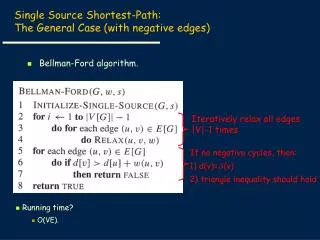
Bellman-Ford algorithm. Iteratively relax all edges |V|-1 times Single Source Shortest-Path: The General Case (with negative edges) • Running time? • O(VE).
Given a directed graph G = (V, E), weight function w : E → R, |V| = n. Assume no negative weight cycles. Goal: create an n × n matrix of shortest-path distances δ(u, v). Could run BELLMAN-FORD once from each vertex: O(V2E)—which is O(V4) if the graph is dense (E = (V2)). If no negative-weight edges, could run Dijkstra’s algorithm once from each vertex: O(V E lg V) with binary heap—O(V3 lg V) if dense, We’ll see how to do in O(V3) in all cases, with no fancy data structure. All-Pairs Shortest Paths
Dynamic programming approach. Use optimal substructure of shortest paths: Any subpath of a shortest path is a shortest path. Create a 3-dimensional table: Let dij(k) –shortest path weight of any path from i to j where all intermediate vertices are from the set {1,2, …, k}. Ultimately, we would like to know the values of dij(n). All Pairs Shortest Path – Floyd-Warshall Algorithm
Base condition: dij(0) = ? dij(0) = wij. For k>0: Let p=<vi, . . . , vj> be a shortest path from vertex i to vertex j with all intermediate vertices in {1,2, …, k}. If k is not an intermediate vertex, then all intermediate vertices are in {1,2, …, k-1}. If k is an intermediate vertex, then p is composed of 2 shortest subpaths drawn from {1,2, …, k-1}. Computing dij(k)
Running time = ? O(n3). Memory required = ? O(n2) (if we drop the superscripts). Algorithm
Idea: If the graph is sparse (|E|<<|V|2), it pays to run Dijkstra’s algorithm once from each vertex. O(VE log V) using binary heap, O(V2 log V + V E) using Fibonacci heap. But Dijkstra’s algorithm does not handle negative edges. Johnson’s Algorithm: reweight edges to form equivalent graph with non-negative edges. Floyd-Warshall still has advantages: very simple implementation no fancy data structures small constant. All-Pairs Shortest Path: Johnson’s Algorithm
Use a graph to model material that flows through conduits. Each edge represents one conduit, and has a capacity, which is an upper bound on the flow rate = units/time. Can think of edges as pipes of different sizes. But flows don’t have to be of liquids. Want to compute max rate that we can ship material from a designated source to a designated sink. The Problem
Each edge (u,v) has a nonnegative capacity c(u,v). If (u,v) is not in E, assume c(u,v)=0. We have a source s, and a sink t. Assume that every vertex v in V is on some path from s to t. c(s,v1)=16; c(v1,s)=0; c(v2,v3)=0 What is a Flow Network?
For each edge (u,v), the flow f(u,v) is a real-valued function that must satisfy 3 conditions: What is a Flow in a Network? • Note that skew symmetry condition implies that f(u,u)=0.
f(v2, v1) = 1, c(v2, v1) = 4. f(v1, v2) = -1, c(v1, v2) = 10. f(v3, s) + f(v3, v1) + f(v3, v2) + f(v3, v4) + f(v3, t) = 0 + (-12) + 4 + (-7) + 15 = 0 flow capacity Example of a Flow:
The value of a flow is given by The Value of a flow • This it the total flow leaving s = the total flow arriving in t.
|f| = f(s, v1) + f(s, v2) + f(s, v3) + f(s, v4) + f(s, t) = 11 + 8 + 0 + 0 + 0 = 19 |f|= f(s, t) + f(v1, t) + f(v2, t) + f(v3, t) + f(v4, t) = 0 + 0 + 0 + 15 + 4 = 19 Example:
We assume that there is only flow in one direction at a time. Sending 7 trucks from Edmonton to Calgary and 3 trucks from Calgary to Edmonton has the same net effect as sending 4 trucks from Edmonton to Calgary. A flow in a network
We have several sources and several targets. Want to maximize the total flow from all sources to all targets. Reduce to max-flow by creating a supersource and a supersink: Multiple Sources Network
Try to improve the flow, until we reach the maximum. The residual capacity of the network with a flow f is given by: The Ford-Fulkerson Method Always nonnegative (why?)
Network: Residual Network: Augmenting path Example of residual capacities
The edges of the residual network are the edges on which the residual capacity is positive. The residual network
An augmenting path p is a simple path from s to t on the residual network. We can put more flow from s to t through p. We call the maximum capacity by which we can increase the flow on p the residual capacity of p. Augmenting Paths
The residual capacity of p = 4. Can improve the flow along p by 4. Augmenting Paths - example
Flow(1) Residual(1) No more augmenting paths max flow attained. Flow(2) Residual(2) Example
The maximum possible flow through the cut = 12 + 7 + 4 = 23 Augmenting Paths – example Flow(2) The network has a capacity of at most 23. This is called a minimum cut.
A cut in a network is a partition of V into S and T=V-S so that s is in S and t is in T. Cuts of Flow Networks
f(S,T) = 12 – 4 + 11 = 19 The net flow through a cut (S,T)
c(S,T)= 12+ 0 + 14 = 26 The capacity of (S,T)
For any cut (S,T), the net flow across (S,T) is f(S,T)=|f|. Lemma 26.5
The value of any flow f in a flow network G is bounded from above by the capacity of any cut of G. Corollary 26.6
If f is a flow in a flow network G=(V,E), with source s and sink t, then the following conditions are equivalent: f is a maximum flow in G. The residual network Gf contains no augmented paths. |f| = c(S,T) for some cut (S,T) (a min-cut). Theorem 26.7 (Max-flow min-cut theorem)
augmenting path Original Network Resulting Flow = Example 4
4 augmenting path Residual Network Resulting Flow = Example
Example Residual Network Resulting Flow = 11
Resulting Flow = 11 augmenting path Residual Network Example
Residual Network Resulting Flow = Example 19
Resulting Flow = 19 augmenting path Residual Network Example
Residual Network Resulting Flow = Example 23
Resulting Flow = 23 No augmenting path: Maxflow=23 Residual Network Example
O(E) O(E) Analysis
If capacities are all integer, then each augmenting path raises |f| by ≥ 1. If max flow is f*, then need ≤ |f*| iterations ⇒ time is O(E|f*|). Note that this running time is not polynomial in input size. It depends on |f*|, which is not a function of |V| or |E|. If capacities are rational, can scale them to integers. If irrational, FORD-FULKERSON might never terminate! Analysis
With time O ( E |f*|), the algorithm is not polynomial. This problem is real: Ford-Fulkerson may perform very badly if we are unlucky: The basic Ford-Fulkerson Algorithm |f*|=2,000,000
Run Ford-Fulkerson on this example Augmenting Path Residual Network