Impact of Stimulus Probability on Response Time and Accuracy in Attention Research
210 likes | 301 Views
This study examines the relationship between stimulus probability and response time/accuracy in attention research using research findings and examples.

Impact of Stimulus Probability on Response Time and Accuracy in Attention Research
E N D
Presentation Transcript
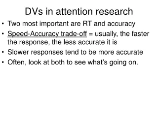
DVs in attention research • Two most important are RT and accuracy • Speed-Accuracy trade-off = usually, the faster the response, the less accurate it is • Slower responses tend to be more accurate • Often, look at both to see what’s going on.
Theios (1975) • Subject named a visually presented digit • DVs were RT and accuracy • IV was stimulus probability (.2 to .8) • Eg, “6” occurs only 20% of the time, but “7” occurs 40% and “9” occurs 80% • Theios found no significant differences in RT • But failed to take into account error rates on the simple task of naming digits.
Interactions: Lorig et al (1991) • DV was event related potentials (ERPs) • High tone on 75% of trials (frequent) • Low tone on 25% of trials (rare) • Observers counted low & ignored high tones • Also varied % musk: 0, 20, (unaware) and 88 (aware).
FIG: Kanto8e 8-12: Lorig et al Effect of varying musk concentration on rare stimuli Effect of varying musk concentration on frequent stimuli
ME’s and INT’s in above Figures: • 2x3 e1: ME of dos. & context, no INT (On the average, percent correct recall (PCR) increased with increasing drug dosage. On the average, PCR was higher for good than poor context. However, the effect of varying context on performance was identical at each level of dosage.)
ME’s and INT’s in above Figures: • 2x3 e2: ME of dos. & context & INT (On the average, PCR increased with increasing dosage. On the average, PCR was higher for good than poor context. Varying context had no effect on PCR when 0 mg of the drug was taken, but had an increasingly differential effect on PCR as the dosage increased.)
ME’s and INT’s in above Figures: • 2x3 e3: ME of dos. & context & INT (On the average, PCR was different when taking the drug than when not taking the drug: Compared to the no-drug condition, PCR was higher when taking 100 mg and lower when taking 200 mg. On the average, PCR was slightly higher for poor than good context. There was a slight advantage in PCR when subjects were given poor context in all but the 200 mg dosage condition.)
ME’s and INT’s in above Figures: • 3x3 e1: ME of dos. & context & INT (On the average, PCR increased with increasing dosage. On the average, PCR increased with improved context for remembering.The advantage of medium context over poor context was identical at all three dosages, however the advantage of good context over both of the other levels of context differed across the levels of drug dosage. Specifically, the advantage of having good context was greater when taking the drug than when not taking the drug.)
ME’s and INT’s in above Figures: • 3x3 e2: ME of dos. & context, no INT (On the average, PCR increased with increasing dosage. On the average, PCR was identical with poor or medium context, but was higher with good context. However, the advantage of good context over the other two levels of context was identical at each level of drug dosage.)
ME’s and INT’s in above Figures: • 3x3 e3: ME of dos. & context & INT (On the average, PCR increased with increasing dosage. On the average, PCR was identical with poor or medium context, but was higher with good context. The advantage of good context over the other two levels of context was identical when the drug was taken, but was greater when no drug was taken.)
ME’s and INT’s in above Figures: • 3x3 e4: ME of dos. & context & INT (On the average, PCR increased with increasing dosage. On the average, PCR was lowest for medium context, slightly higher for poor context, and highest for good context. For the placebo group, medium context led to slightly higher PCR than poor context, and good context led to much better PCR than the other two levels of context. This advantage of good context over the other two levels of context was reduced for the 100 mg group, and there was no difference in PCR between poor and medium context. For the 200 mg group, there was an advantage in PCR for good context over poor context, and an even greater advantage over medium context.)
ME’s and INT’s in above Figures: • 3x3 e5: no ME of dos or context, but INT (On the average, PCR was the same across all three drug groups, and was the same for all three levels of context. However, the lack of two significant main effects was obscured by the presence of a complex cross-over interaction, in which increasing the drug dosage improved PCR for those with poor context, harmed PCR for those with medium context, and had no effect on PCR for those with good context.)