Download
1 / 24
260 likes | 438 Views
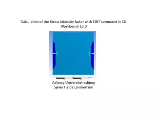
Calculation of the Stress intensity factor with CINT command in 3D Workbench 13.0 Aalborg Universitet esbjerg Søren Heide Lambertsen. Start a new Static Structural. Chose mm as length unit. Build the geometry and model the crack. The crack on this side is made with a ellipse.

E N D
Calculation of the Stress intensity factor with CINT command in 3D Workbench 13.0 Aalborg Universitet esbjerg Søren Heide Lambertsen
The model is sliced in two parts to get a better mesh control.
Stress distribution is not as it is expected and the deformation of the crack either. The problem is that workbench sometime add contact elements automatically and these had to be removed.
Now the stress and deformation is more as it is expected to be.
Then add a coordinate system for each crack. It is important that the y axis is normal to the crack plane. Also add a name for the coordinate system, in this example the name 44 is used
Then add a commands (APDL) under static structural. In the 2d crack tutorials there is a detail description of the commands.
The commands: CINT,new,1 ! CINT ID number. CINT,type,sifs ! Type of calculation CINT,norm,5 ! Number of contours to be calculated. CINT,ctnc,tip1 ! Crack tip node component name CINT,ncon,33,2 ! Coordinate system number and Axis of coordinate system CINT,new,2 CINT,type,sifs CINT,norm,5 CINT,ctnc,tip2 CINT,ncon,44,2
And then add a commands (APDL) to the solution and enter the commands to plot the results.
The commands: /show,png ! Show the PNG files PLCINT, front,1,,,k1 ! Plot result from the CINT commands id 1 the value of k1 PLCINT, front,2,,,k1 ! Plot result from the CINT commands id 2 the value of k1 It is also possible to print the result in the solution information window by the command: PRCINT
PLCINT command is shown under the commands (APDL). By the result it is clear that the path 1 give a bad calculation and path 2,3,4,5 gives a better result. Because of the finite element approximation, the value of k1 is different for each path. The first path for K1 is best discarded since it contains the singularity. The true value of K is usually estimated as the average of the remaining paths.
Crack calculation 2 gives a bad result. The reason is often that the y axis has to be switch because the J integral gives a negative result and therefore the K1 calculation is incorrect.
The coordinate system is changed, the contour number is set to 10.