Inference about Population Parameters: Hypothesis Testing

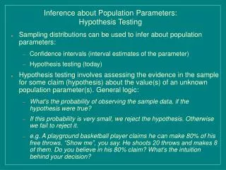
1. Inference about Population Parameters:Hypothesis Testing • Sampling distributions can be used to infer about population parameters: • Confidence intervals (interval estimates of the parameter) • Hypothesis testing (today) • Hypothesis testing involves assessing the evidence in the sample for some claim (hypothesis) about the value(s) of an unknown population parameter(s). General logic: • What's the probability of observing the sample data, if the hypothesis were true? • If this probability is very small, we reject the hypothesis. Otherwise we fail to reject it. • e.g. A playground basketball player claims he can make 80% of his free throws. “Show me”, you say. He shoots 20 throws and makes 8 of them. Do you believe in his 80% claim? What's the intuition behind your decision?

2. The Null and Alternative Hypotheses • The Null Hypothesis, H0 : The claim about the population parameter(s) we want to test. Examples of H0: • The population proportion/mean equals certain value • No difference in the means of two groups • No relationship between two variables • The “alternative hypothesis”, Ha, is the alternative statement about the population parameter(s) instead of H0. Often Hais what we suspect or hope is true.

3. Elements of Hypothesis Testing • Determine the two hypotheses • Compute the observed value of the test statistic, which is some sample statistic (such as sample proportion or sample mean) that has a known sampling distribution under the null hypothesis. • Using this sampling distribution, determine how (un)likely it is to observe the test statistic taking values as extreme as observed or more so, if the null hypothesis were true (i.e., find the “p-value”) • Make a decision/conclusion based on the p-value: based on the observed sample statistic, shall we reject the null hypothesis? (Or, do we consider the computed p-value “small” enough?) • e.g. The basketball case (testing hypothesis about a proportion) • You may want to explore http://www.whfreeman.com/scc7e

4. Testing Hypotheses about a Population Proportion:Stating the hypotheses • Null: H0: p=p0 • One sided alternatives (for “one tailed test”) Ha: p>p0 Ha: p<p0 • Two sided alternative (for “two tailed test”) Ha: pp0

5. Testing Hypotheses about a Population Proportion:Computing the test statistic and determining its sampling distribution under the null hypothesis • Quite intuitively, our test statistic for testing the population proportion is the sample proportion, • Recall the sampling distribution of the sample proportion: approximately normal with mean p and standard deviation • Under the null hypothesis (i.e., assuming the null hypothesis is true), p=p0, so the sample proportion follows a normal distribution with p replaced by p0 • Which means:

6. Testing Hypotheses about a Population Proportion:Finding the p-value of the test statistic • Using the sampling distribution of the sample proportion under the null hypothesis, we can find out the probability of observing a sample proportion value as extreme as in our data or more so. • A small p-value indicates that the observed data (or relationship) is unlikely to have occurred if the null hypothesis were actually true • The p-value tends to be small when there is evidence in the data against the null hypothesis

7. Finding the P-value for Testing Proportions • For one tailed test, the p-value is the area in theright tail if the alternative hypothesis takes the form Ha: p>p0i.e., The p-value is the probability of getting a value as large or larger than the observed test statistic value. (Left tail if Ha: p<p0) • For two tailed test, the p-value is the sum of the areas in both tails. i.e., The p-value is the probability of getting a value as far away (or farther) from the mean as the absolute value of the observed test statistic (z) value. (Doubles the p-value from one tailed test). • Using Stata: Statistics-->Summaries, tables, and tests --> classical tests of hypotheses, or “prtest”

8. P-value for Testing Proportions: H0: p=p0; Ha: p>p0 Example: p0=0.5, n=50, # success=28 (or 36)

9. P-value for Testing Proportions:H0: p=p0; Ha: pp0 Example: p0=0.5, n=4040, # success=2048

10. Testing Hypotheses about a Population Proportion:Making a decision based on the p-value • If we think the P-value istoo low for the observed test statistic to lend support/evidence for the null hypothesis, then we would reject the null hypothesis; otherwise, we fail to reject the null hypothesis. • When the null hypothesis takes the form of having no relationship or no difference, our rejection of it would mean that we found evidence that there is astatistically significantrelationship/difference. • In general, we say that:

11. Typical Cut-off for the P-value • So how small is “small”? • Typically, a p-value less than 0.05 is considered to be small enough to lead us to reject the null hypothesis. • Some researchers use 0.10 or 0.01 as the cut-off instead of 0.05. • This “cut-off” value is typically referred to as the significance level  of the test.  is also referred to as the “type I error” of the test. It is the probability of rejecting the null hypothesis when it is true. • If we decide not to reject the null, we risk the “type II error”, which is the probability of failing to reject the null when it is false (its size depends on a, as well as the “true” parameter value and sample size.) • (1-type II error) is defined as the power of the test. • Recommendation: always report the actual p-value, in addition to (or even instead of) reporting “significance at the .05 level”.

12. Testing Hypotheses about a Population Mean • The idea is exactly the same as the proportion case. The test statistic now involves the sample mean, which has a slightly different form of sampling distribution from the proportion, as we have seen last time. That's all. • Same logic, same procedure • e.g. National Assessment of Educational Progress (NAEP) quantitative test scores for young men aged 21-25. (Score can range from 0-500). Says a score of 275 or higher reflects the skills needed to balance a check book. • A random sample of 840 men 21-25 yrs of age has a sample mean of 272, and sample s.d. Of 59. • Do we have enough evidence to say that the mean score in the population of all 9.5 million young men in this age group is less than 275? • H0:m=275; Ha:m<275 • Under H0, the sample mean follows • N(275, 59/sqrt(840))=N(275,2.036). • Z=(272-275)/2.036=-1.47

13. Testing Hypotheses about a Population Mean The shaded area is about .07, which is the p-value. Would you reject the null hypothesis?

14. Testing Hypotheses about a Population Mean: a two tailed test example Executives' blood pressure different from the national mean of 128? H0: m=128; Ha: m128. Sample mean is 126.1, s=15.2, n=72. Z=-1.06.The shaded area is about .27, which is the p-value. Would you reject the null hypothesis?

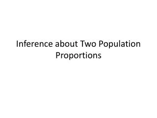
15. Comparing two Proportions (or Means) • The logic and procedure are exactly the same as the single parameter case, only that now we need to make use of the sampling distribution of the difference between two proportions (or means), which turns out also to be normal, with mean being the difference of the population proportions (or means), and standard deviation computable through a simple formula • Under the null hypothesis that the two population proportions are the same, the mean of the sampling distribution is 0. • Thus, upon observing two sample proportions/means, one can take the difference of them, and use the sampling distribution to find out the p-value under the null hypothesis, then make a decision to reject the null or not. • In Stata, choose “two sample” tests. Or use by() option for “prtest” or “ttest” • e.g., gss2002.dta, prtest vote00, by(born)