Losslessy Compression of Multimedia Data
260 likes | 624 Views
Losslessy Compression of Multimedia Data. Hao Jiang Computer Science Department Sept. 25, 2007. Lossy Compression. Apart from lossless compression, we can further reduce the bits to represent media data by discarding “unnecessary” information.

Losslessy Compression of Multimedia Data
E N D
Presentation Transcript
Losslessy Compression of Multimedia Data Hao Jiang Computer Science Department Sept. 25, 2007
Lossy Compression • Apart from lossless compression, we can further reduce the bits to represent media data by discarding “unnecessary” information. • Media such as image, audio and video can be “modified” without seriously affecting the perceived quality. • Lossy multimedia data compression standards include JPEG, MPEG, etc.
Methods of Discarding Information • Reducing resolution Original image 1/2 resolution and zoom in
Reduce pixel color levels Original image ½ color levels
For audios and videos we can similarly reduce the sampling rate, the sample levels, etc. • These methods usually introduce large distortion. Smarter schemes are necessary! 2.3bits/pixel (JPEG)
Distortion • Distortion: the amount of difference between the encoded media data and the original one. • Distortion measurement • Mean Square Error (MSE) mean( ||xorg – xdecoded||2) • Signal to Noise Ratio (SNR) SNR = 10log10 (Signal_Power)/(MSE) (dB) • Peak Signal to Noise Ratio PSNR = 10log10(255^2/MSE) (dB)
The Relation of Rate and Distortion • The lowest possible rate (average codeword length per symbol) is correlated with the distortion. Bit Rate H 0 D_max D
Quantization • Maps a continuous or discrete set of values into a smaller set of values. • The basic method to “throw away” information. • Quantization can be used for both scalars (single numbers) or vectors (several numbers together). • After quantization, we can generate a fixed length code directly.
Uniform Scalar Quantization Assume x is in [xmin, xmax]. We partition the interval uniformly into N nonoverlapping regions. Quantization step D =(xmax-xmin)/N xmin xmax Quantization value Decision boundaries A quantizer Q(x) maps x to the quantization value in the region where x falls in.
Quantization Example Q(x) = [floor(x/D) + 0.5] D Q(x)/ D 2.5 1.5 0.5 -3 -2 -1 0 1 2 3 x/D -0.5 -1.5 -2.5 Midrise quantization
Quantization Example Q(x) = [round(x/D)] D Q(x)/ D 3 2 1 -3 -2 -1 0 1 2 3 x/D -1 -2 -3 Midrise quantization
Quantization Error • To minimize the possible maximum error, the quantization value should be at the center of each decision interval. • If x randomly occurs, Q(x) is uniformly distributed in [-D/2, D/2] Quantization error xn+1 xn x Quantization value
Quantization and Codewords 001 010 011 100 101 000 xmin xmax Each quantization value can be associated with a binary codeword. In the above example, the codeword corresponds to the index of each quantization value.
Another Coding Scheme • Gray code 000 001 011 010 110 111 xmin xmax • The above codeword is different in only 1bit • for each neighbors. • Gray code is more resistant to bit errors than the • natural binary code.
Bit Assignment • If the # of quantization interval is N, we can use log2(N) bits to represent each quantized value. • For uniform distributed x, The SNR of Q(x) is proportional to 20log(N) = 6.02n, where N=2n dB About 6db gain 1 more bit bits
Non-uniform Quantizer • For audio and visual, the tolerance of a distortion is proportional to the signal size. • So, we can make quantization step D proportional to the signal level. • If signal is not uniformly distributed, we also prefer non-uniform quantization. Perceived distortion ~ D / s 0
Vector Quantization Decision Region Quantization Value
Predictive Coding … - - - - + + + + 1 2 1 1 -2 -1 -1 -1 3 1 1 1 1 + • Lossless difference coding revisited encoder 0 1 3 4 5 3 2 1 0 3 4 5 6 7 0 … + + 1 3 4 5 3 2 1 0 3 4 5 6 7 decoder
Predictive Coding in Lossy Compression 1 3 4 5 3 2 1 0 3 4 5 6 7 1 1 1 1 -1 -1 -1 -1 1 1 1 1 1 Encoder 0 - + + + + - - - … Q Q Q Local decoder … + + + 0 1 2 3 4 3 2 1 0 1 2 3 4 5 Q(x) = 1 if x > 0, 0 if x == 0 and –1 if x < 0
A Different Notation Entropy coding Audio samples or image pixels + - 0101… Buffer Lossless Predictive Encoder Diagram
A Different Notation Entropy decoding Reconstructed audio samples or image pixels Code stream + + Buffer Lossless Predictive Decoder Diagram
A different Notation Lossy Predictive Coding 0101… Coding Audio samples or image pixels Q + - Local Decompression + Buffer
General Prediction Method • For image: • For Audio: • Issues with Predictive Coding • Not resistant to bit errors. • Random access problem. C B A X D C B A X
Transform Coding + + + + + + + + + + + + 1 3 4 5 3 2 1 0 3 4 5 6 ½ ½ ½ ½ ½ ½ 2 4.5 2.5 0.5 3.5 5.5 1 3 4 5 3 2 1 0 3 4 5 6 - - - - - - ½ ½ ½ ½ ½ ½ -1 -0.5 0.5 0.5 -0.5 0.5
Transform and Inverse Transform We did a transform for a block of input data using x1 x2 y1 y2 ½ ½ ½ -½ = The inverse transform is: y1 y2 x1 x2 1 1 1 -1 =
Transform Coding • A proper transform focuses the energy into small number of numbers. • We can then quantize these values differently and achieve high compression ratio. • Useful transforms in compressing multimedia data: • Fourier Transform • Discrete Cosine Transform